Análisis de datos espaciales en R

Manejo de datos espaciales en R

Diego Nieto Lugilde

Universidad de Córdoba (España)

Introducción a los datos espaciales

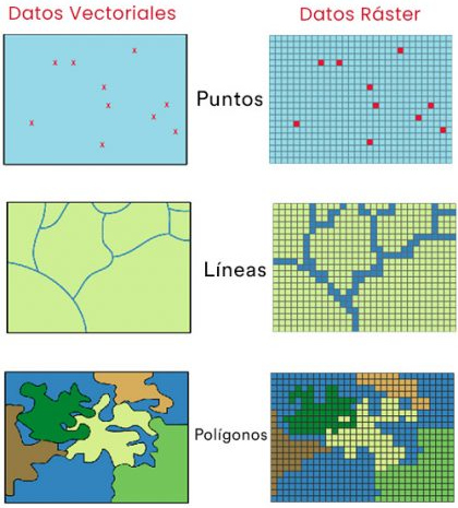
¿Qué son los datos espaciales?

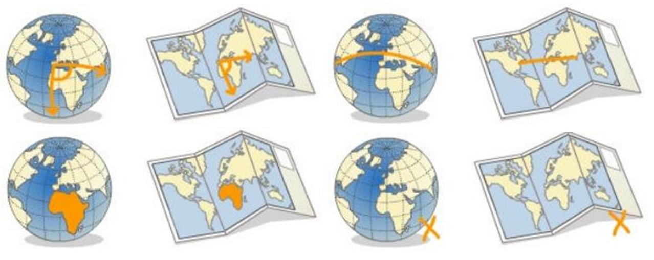
La misma información se puede representar de varias maneras

Algunos tipos de datos se ajustan mejor a ciertas formas de representación

¿Cómo se localiza la información?

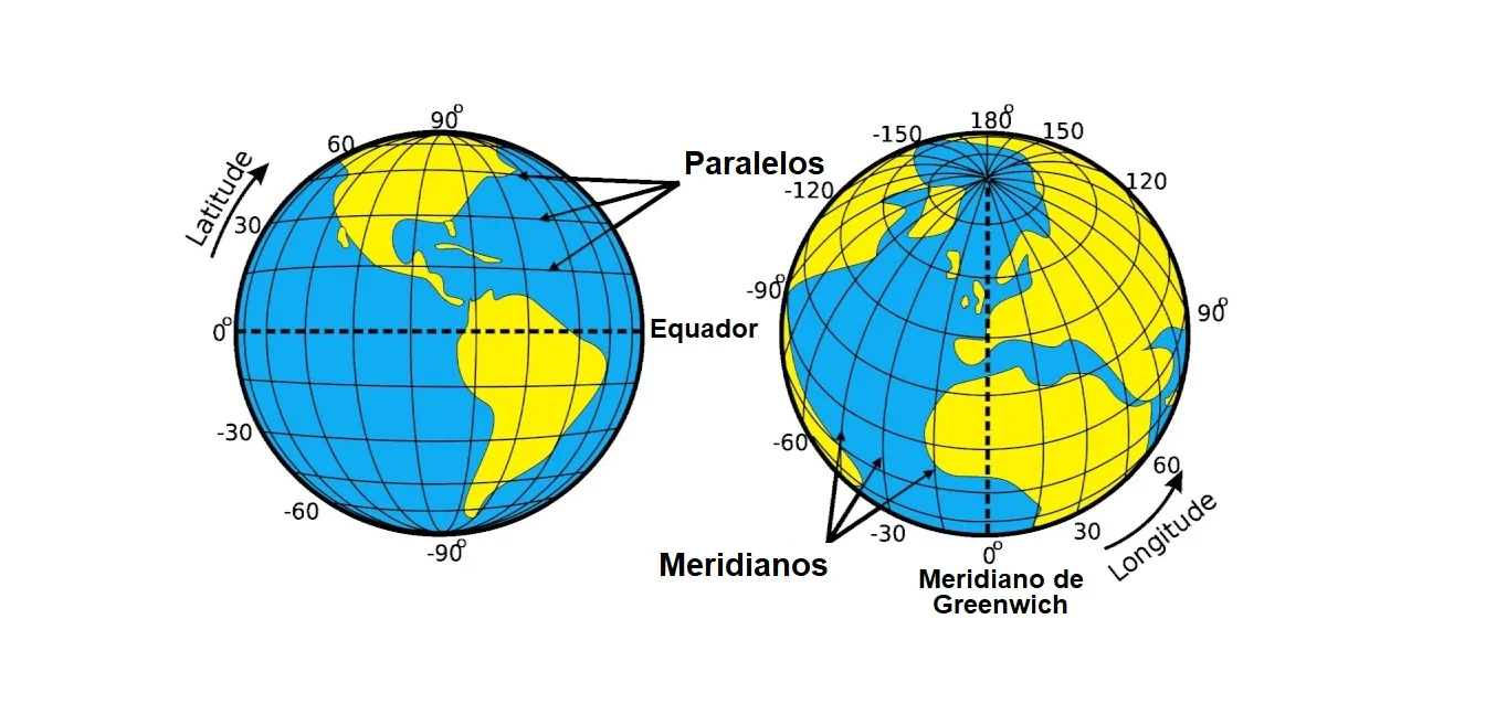
No parece fácil medir los ángulos ;)

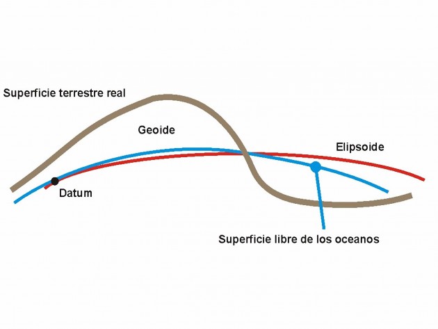
Se calculan aproximaciones usando modelos de la Tierra (Datum)

No es lo mismo saber donde ocurre algo que dibujarlo en un mapa

Para ello es necesario proyectar una esfera sobre un plano

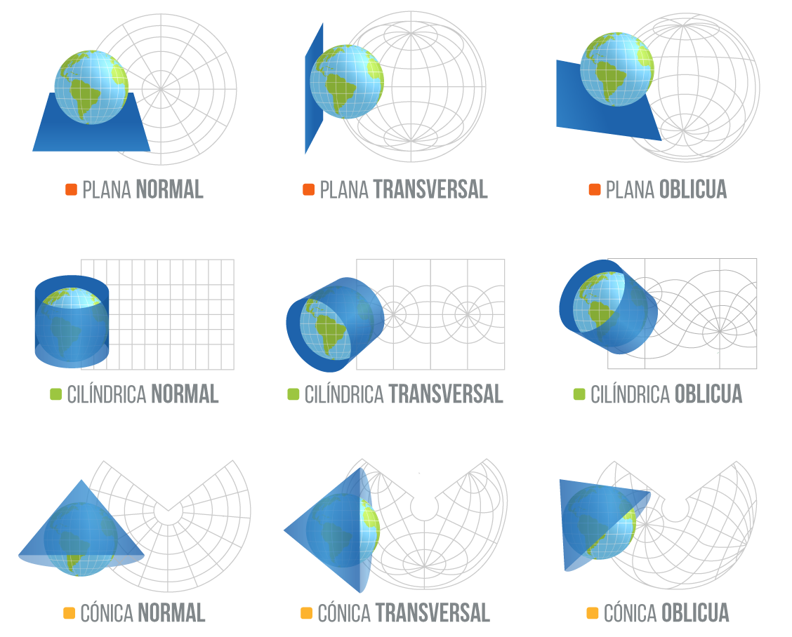
Cada proyección y cada datum genera mapas con propiedades diferentes

Conformes, equidistantes, equivalentes y afilácticas

Manejando datos espaciales

Vamos a usar el paquete terra

# install.packages("terra")
library(terra)

Manejando datos vectoriales

Podemos crear datos vectoriales desde cero

Los más sencillos de crear son los puntos

lon <- c(-116.7, -120.4, -116.7, -113.5, -115.5, -120.8, -119.5, -113.7, -113.7, -110.7) 
lat <- c(45.3, 42.6, 38.9, 42.1, 35.7, 38.9, 36.2, 39, 41.6, 36.9) 
lonlat <- cbind(lon, lat) 
pts <- vect(lonlat) 
pts

 class       : SpatVector 
 geometry    : points 
 dimensions  : 10, 0  (geometries, attributes)
 extent      : -120.8, -110.7, 35.7, 45.3  (xmin, xmax, ymin, ymax)
 coord. ref. :  

Warning

Fijaros que el apartado “coord. ref.” está vacío

Revisamos el tipo de datos

class(pts)

[1] "SpatVector"
attr(,"package")
[1] "terra"

geom(pts)

      geom part      x    y hole
 [1,]    1    1 -116.7 45.3    0
 [2,]    2    1 -120.4 42.6    0
 [3,]    3    1 -116.7 38.9    0
 [4,]    4    1 -113.5 42.1    0
 [5,]    5    1 -115.5 35.7    0
 [6,]    6    1 -120.8 38.9    0
 [7,]    7    1 -119.5 36.2    0
 [8,]    8    1 -113.7 39.0    0
 [9,]    9    1 -113.7 41.6    0
[10,]   10    1 -110.7 36.9    0

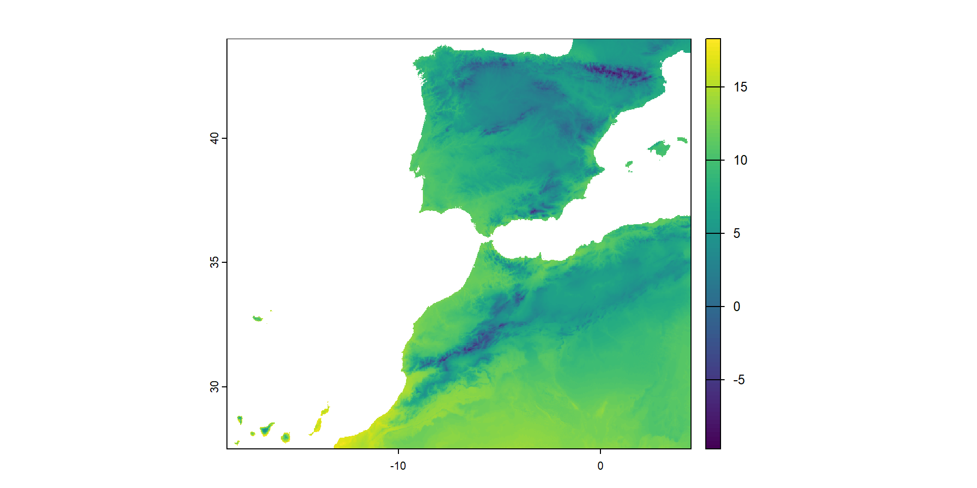
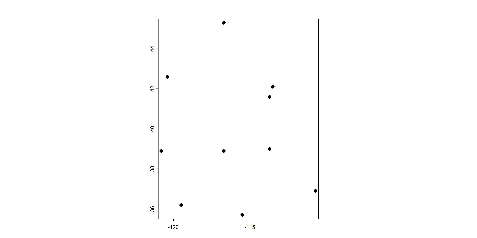
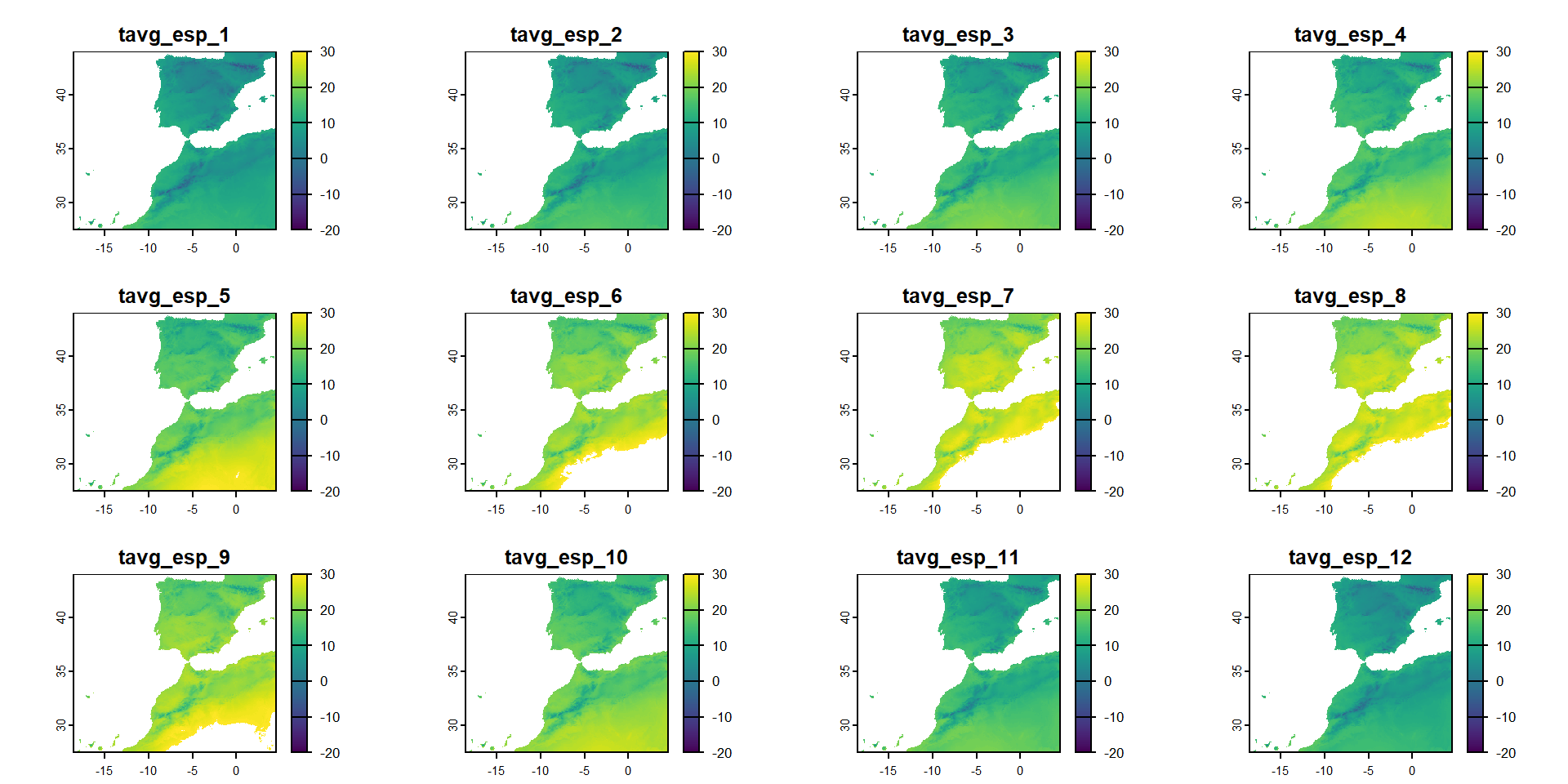
Veamos la distribución espacial de los datos

plot(pts)

Definimos el sistema de referencia de coordenadas (CRS)

crdref <- "+proj=longlat +datum=WGS84"
pts <- vect(lonlat, crs = crdref)
pts

 class       : SpatVector 
 geometry    : points 
 dimensions  : 10, 0  (geometries, attributes)
 extent      : -120.8, -110.7, 35.7, 45.3  (xmin, xmax, ymin, ymax)
 coord. ref. : +proj=longlat +datum=WGS84 +no_defs 

Podemos comprobar el CRS de un objeto vectorial

crs(pts)

[1] "GEOGCRS[\"unknown\",\n    DATUM[\"World Geodetic System 1984\",\n        ELLIPSOID[\"WGS 84\",6378137,298.257223563,\n            LENGTHUNIT[\"metre\",1]],\n        ID[\"EPSG\",6326]],\n    PRIMEM[\"Greenwich\",0,\n        ANGLEUNIT[\"degree\",0.0174532925199433],\n        ID[\"EPSG\",8901]],\n    CS[ellipsoidal,2],\n        AXIS[\"longitude\",east,\n            ORDER[1],\n            ANGLEUNIT[\"degree\",0.0174532925199433,\n                ID[\"EPSG\",9122]]],\n        AXIS[\"latitude\",north,\n            ORDER[2],\n            ANGLEUNIT[\"degree\",0.0174532925199433,\n                ID[\"EPSG\",9122]]]]"

La ubicación sola no es muy interesante…

Voy a simular valores de precipitación al azar (sample), un valor para cada punto

precipvalue <- sample(1:100, 10)
df <- data.frame(ID = 1:nrow(lonlat), 
                 precip = precipvalue)
pts <- vect(lonlat, atts = df, crs = crdref)
pts

 class       : SpatVector 
 geometry    : points 
 dimensions  : 10, 2  (geometries, attributes)
 extent      : -120.8, -110.7, 35.7, 45.3  (xmin, xmax, ymin, ymax)
 coord. ref. : +proj=longlat +datum=WGS84 +no_defs 
 names       :    ID precip
 type        : <int>  <int>
 values      :     1     81
                   2     61
                   3     26

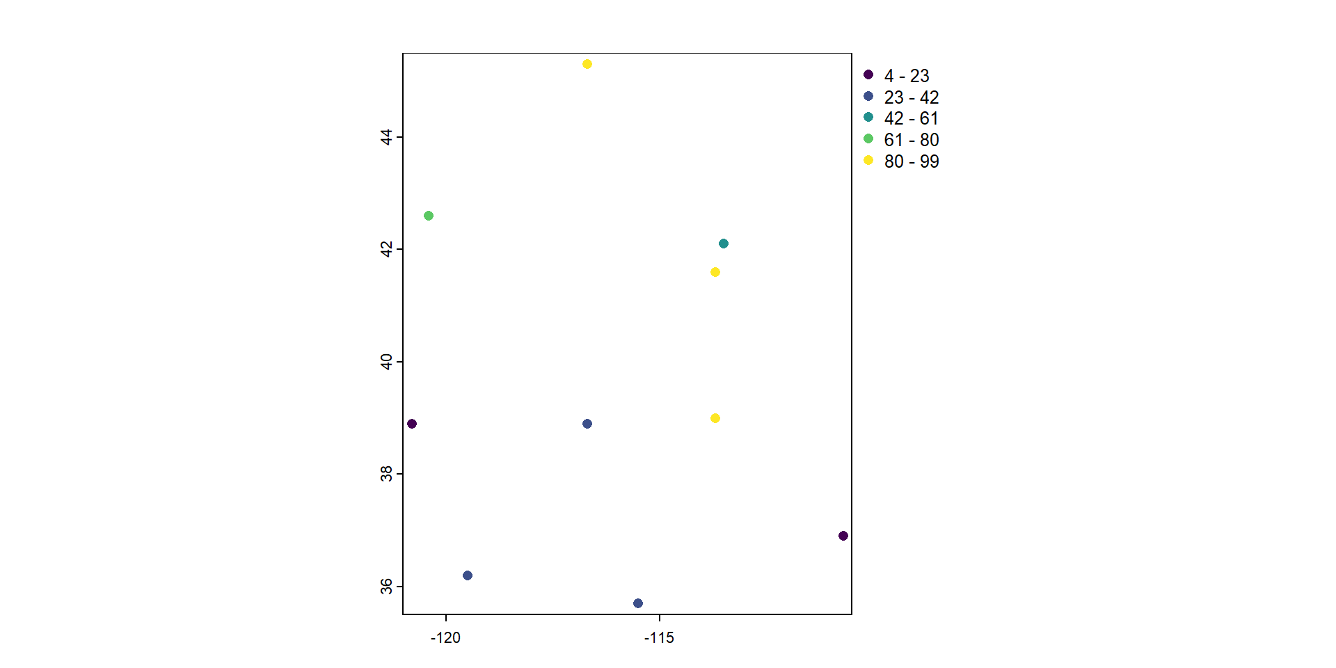
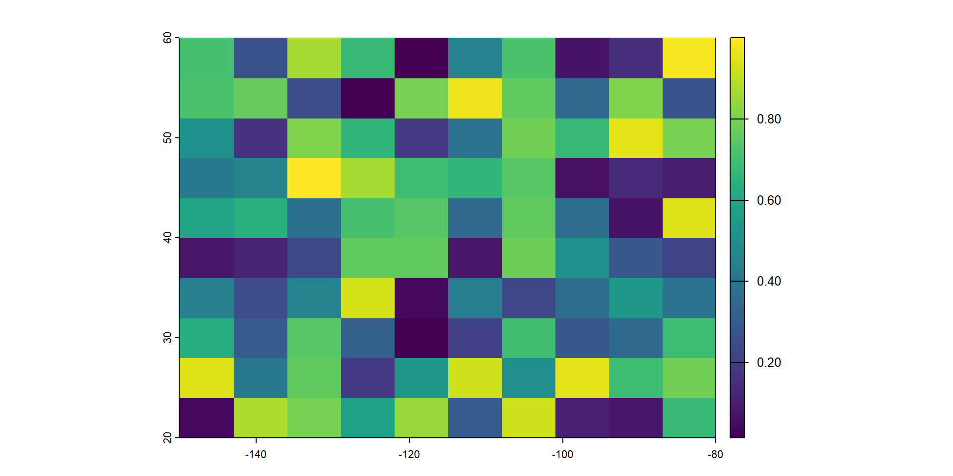
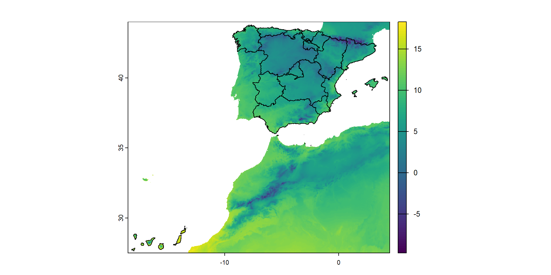
Veamos las precipitaciones en su contexto espacial

plot(pts, "precip", type = "interval")

Vamos a generar ahora un segundo conjunto de puntos…

lon2 <- c(-116.8, -114.2, -112.9, -111.9, -114.2, -115.4, -117.7)
lat2 <- c(41.3, 42.9, 42.4, 39.8, 37.6, 38.3, 37.6)
lonlat2 <- cbind(id = c(1,1,1,1,1,1,1), part = c(1,1,1,1,1,1,1), lon2, lat2)
lonlat2

     id part   lon2 lat2
[1,]  1    1 -116.8 41.3
[2,]  1    1 -114.2 42.9
[3,]  1    1 -112.9 42.4
[4,]  1    1 -111.9 39.8
[5,]  1    1 -114.2 37.6
[6,]  1    1 -115.4 38.3
[7,]  1    1 -117.7 37.6

… pero para crear datos de líneas…

lns <- vect(lonlat2, type = "lines", crs = crdref)
lns

 class       : SpatVector 
 geometry    : lines 
 dimensions  : 1, 0  (geometries, attributes)
 extent      : -117.7, -111.9, 37.6, 42.9  (xmin, xmax, ymin, ymax)
 coord. ref. : +proj=longlat +datum=WGS84 +no_defs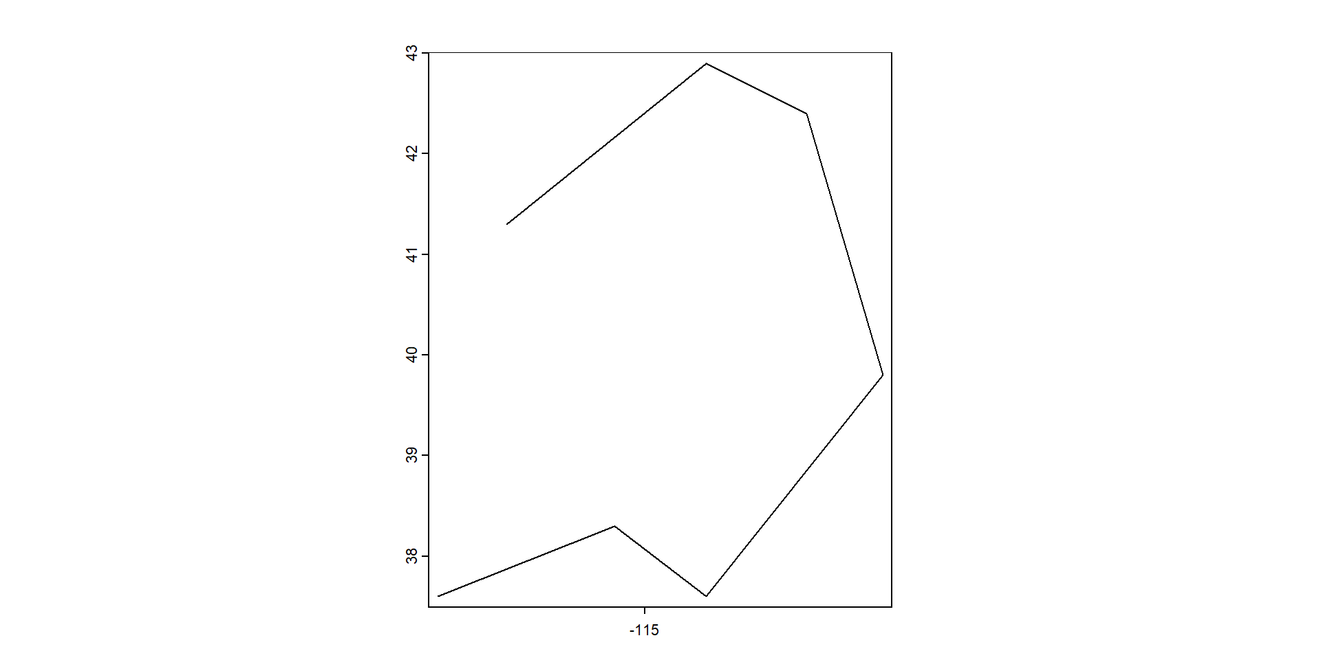 

plot(lns)

… o un datos de polígonos

pols <- vect(lonlat2, type = "polygons", crs = crdref)
pols

 class       : SpatVector 
 geometry    : polygons 
 dimensions  : 1, 0  (geometries, attributes)
 extent      : -117.7, -111.9, 37.6, 42.9  (xmin, xmax, ymin, ymax)
 coord. ref. : +proj=longlat +datum=WGS84 +no_defs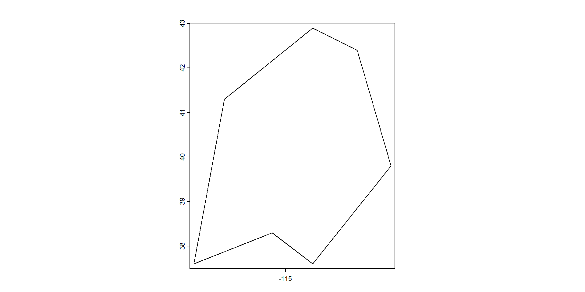 

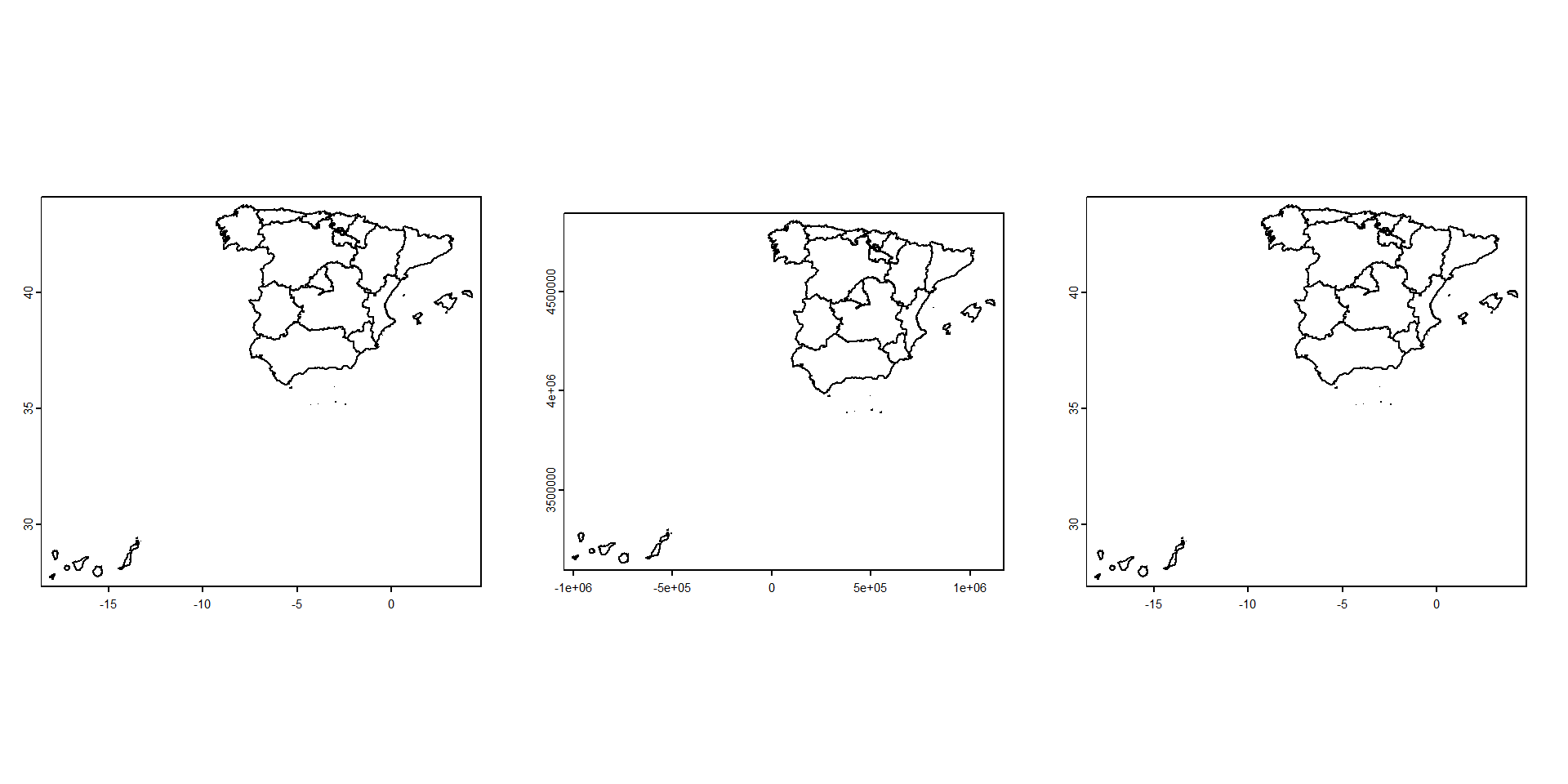
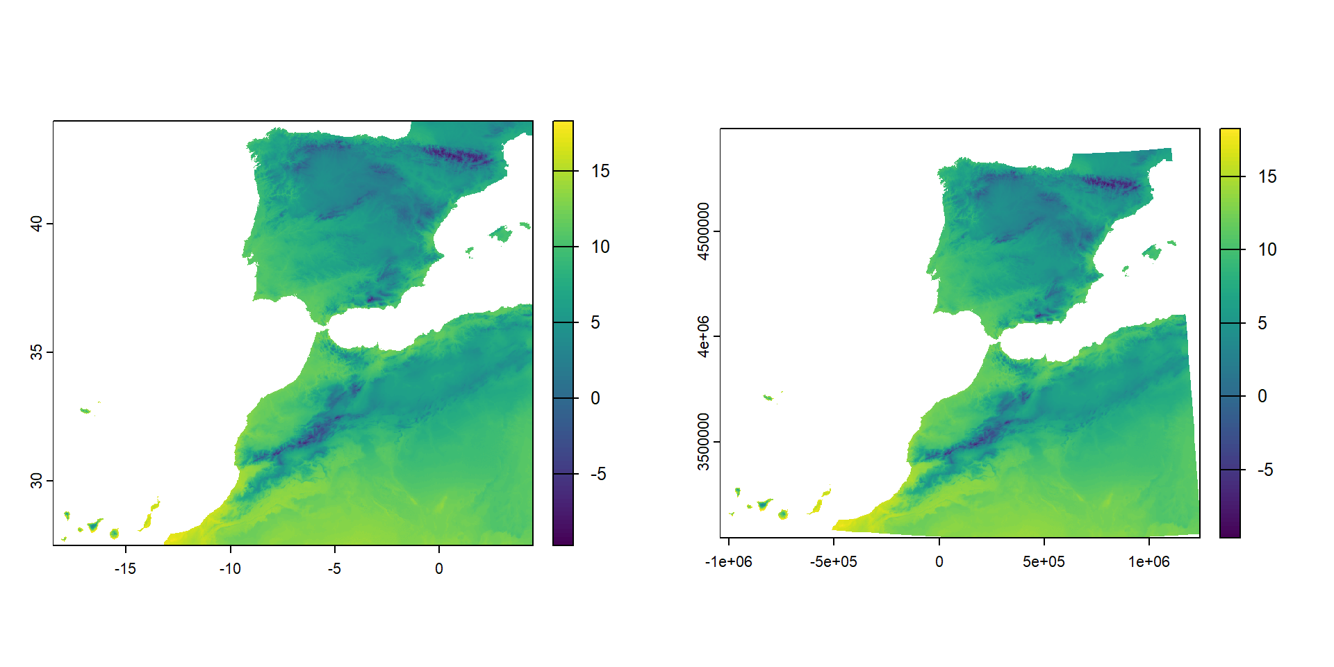
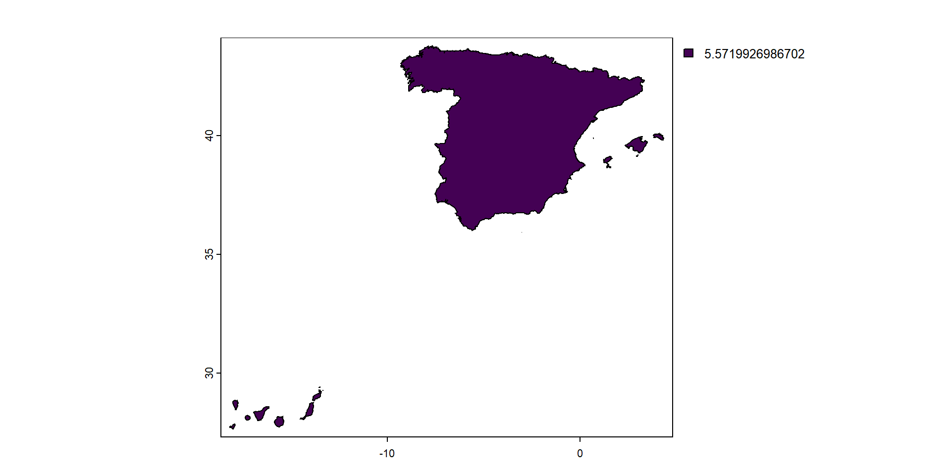
plot(pols)

Lo más normal es usar datos generados con un SIG

Descargar datos de Internet (v.gr. GADM) y cargarlos desde el disco duro

esp <- vect("data/gadm/gadm41_ESP_1.shp")
esp

Lo más normal es usar datos generados con un SIG

Hay paquetes de R que dan acceso directo a datos vectoriales (v.gr. geodata)

# install.packages("geodata")
library(geodata)
esp <- gadm("ESP", level = 1, path = ".")
esp

 class       : SpatVector 
 geometry    : polygons 
 dimensions  : 18, 11  (geometries, attributes)
 extent      : -18.16153, 4.328195, 27.63736, 43.79153  (xmin, xmax, ymin, ymax)
 coord. ref. : lon/lat WGS 84 (EPSG:4326) 
 names       :   GID_1 GID_0 COUNTRY    NAME_1       VARNAME_1 NL_NAME_1
 type        :   <chr> <chr>   <chr>     <chr>           <chr>     <chr>
 values      : ESP.1_1   ESP   Spain Andalucía Andalousie|And~        NA
               ESP.2_1   ESP   Spain    Aragón Aragão|Aragó|A~        NA
               ESP.3_1   ESP   Spain Cantabria Cantàbria|Cant~        NA
          TYPE_1       ENGTYPE_1  CC_1 HASC_1 ISO_1
           <chr>           <chr> <chr>  <chr> <chr>
 Comunidad Autó~ Autonomous Com~    01  ES.AN    NA
 Comunidad Autó~ Autonomous Com~    15  ES.AR    NA
 Comunidad Autó~ Autonomous Com~    06  ES.CB ES-CB

Veamos si se parece a lo que conocemos…

plot(esp)

Estos datos se pueden guardar para no tener que volver a descargarlos

writeVector(esp, "esp.shp", overwrite = TRUE)

Comprobemos el CRS de alguno de nuestros datos

crs(esp)

[1] "GEOGCRS[\"WGS 84\",\n    DATUM[\"World Geodetic System 1984\",\n        ELLIPSOID[\"WGS 84\",6378137,298.257223563,\n            LENGTHUNIT[\"metre\",1]]],\n    PRIMEM[\"Greenwich\",0,\n        ANGLEUNIT[\"degree\",0.0174532925199433]],\n    CS[ellipsoidal,2],\n        AXIS[\"geodetic latitude (Lat)\",north,\n            ORDER[1],\n            ANGLEUNIT[\"degree\",0.0174532925199433]],\n        AXIS[\"geodetic longitude (Lon)\",east,\n            ORDER[2],\n            ANGLEUNIT[\"degree\",0.0174532925199433]],\n    ID[\"EPSG\",4326]]"

Se puede borrar el CRS del conjunto de datos

esp_sin_crs <- esp
crs(esp_sin_crs) <- ""
crs(esp_sin_crs)

[1] ""

O se puede especificar a mano (estandar PROJ.4)

esp_falso_utm <- esp
crs(esp_falso_utm) <- "+proj=utm +zone=19 +south +datum=WGS84 +units=m +no_defs +type=crs"
crs(esp_falso_utm)

[1] "PROJCRS[\"unknown\",\n    BASEGEOGCRS[\"unknown\",\n        DATUM[\"World Geodetic System 1984\",\n            ELLIPSOID[\"WGS 84\",6378137,298.257223563,\n                LENGTHUNIT[\"metre\",1]],\n            ID[\"EPSG\",6326]],\n        PRIMEM[\"Greenwich\",0,\n            ANGLEUNIT[\"degree\",0.0174532925199433],\n            ID[\"EPSG\",8901]]],\n    CONVERSION[\"UTM zone 19S\",\n        METHOD[\"Transverse Mercator\",\n            ID[\"EPSG\",9807]],\n        PARAMETER[\"Latitude of natural origin\",0,\n            ANGLEUNIT[\"degree\",0.0174532925199433],\n            ID[\"EPSG\",8801]],\n        PARAMETER[\"Longitude of natural origin\",-69,\n            ANGLEUNIT[\"degree\",0.0174532925199433],\n            ID[\"EPSG\",8802]],\n        PARAMETER[\"Scale factor at natural origin\",0.9996,\n            SCALEUNIT[\"unity\",1],\n            ID[\"EPSG\",8805]],\n        PARAMETER[\"False easting\",500000,\n            LENGTHUNIT[\"metre\",1],\n            ID[\"EPSG\",8806]],\n        PARAMETER[\"False northing\",10000000,\n            LENGTHUNIT[\"metre\",1],\n            ID[\"EPSG\",8807]],\n        ID[\"EPSG\",17019]],\n    CS[Cartesian,2],\n        AXIS[\"(E)\",east,\n            ORDER[1],\n            LENGTHUNIT[\"metre\",1,\n                ID[\"EPSG\",9001]]],\n        AXIS[\"(N)\",north,\n            ORDER[2],\n            LENGTHUNIT[\"metre\",1,\n                ID[\"EPSG\",9001]]]]"

O se puede especificar con los códigos EPSG

esp_false_utm2 <- esp
crs(esp_false_utm2) <- "EPSG:3042"
crs(esp_false_utm2)

[1] "PROJCRS[\"ETRS89 / UTM zone 30N (N-E)\",\n    BASEGEOGCRS[\"ETRS89\",\n        ENSEMBLE[\"European Terrestrial Reference System 1989 ensemble\",\n            MEMBER[\"European Terrestrial Reference Frame 1989\"],\n            MEMBER[\"European Terrestrial Reference Frame 1990\"],\n            MEMBER[\"European Terrestrial Reference Frame 1991\"],\n            MEMBER[\"European Terrestrial Reference Frame 1992\"],\n            MEMBER[\"European Terrestrial Reference Frame 1993\"],\n            MEMBER[\"European Terrestrial Reference Frame 1994\"],\n            MEMBER[\"European Terrestrial Reference Frame 1996\"],\n            MEMBER[\"European Terrestrial Reference Frame 1997\"],\n            MEMBER[\"European Terrestrial Reference Frame 2000\"],\n            MEMBER[\"European Terrestrial Reference Frame 2005\"],\n            MEMBER[\"European Terrestrial Reference Frame 2014\"],\n            ELLIPSOID[\"GRS 1980\",6378137,298.257222101,\n                LENGTHUNIT[\"metre\",1]],\n            ENSEMBLEACCURACY[0.1]],\n        PRIMEM[\"Greenwich\",0,\n            ANGLEUNIT[\"degree\",0.0174532925199433]],\n        ID[\"EPSG\",4258]],\n    CONVERSION[\"UTM zone 30N\",\n        METHOD[\"Transverse Mercator\",\n            ID[\"EPSG\",9807]],\n        PARAMETER[\"Latitude of natural origin\",0,\n            ANGLEUNIT[\"degree\",0.0174532925199433],\n            ID[\"EPSG\",8801]],\n        PARAMETER[\"Longitude of natural origin\",-3,\n            ANGLEUNIT[\"degree\",0.0174532925199433],\n            ID[\"EPSG\",8802]],\n        PARAMETER[\"Scale factor at natural origin\",0.9996,\n            SCALEUNIT[\"unity\",1],\n            ID[\"EPSG\",8805]],\n        PARAMETER[\"False easting\",500000,\n            LENGTHUNIT[\"metre\",1],\n            ID[\"EPSG\",8806]],\n        PARAMETER[\"False northing\",0,\n            LENGTHUNIT[\"metre\",1],\n            ID[\"EPSG\",8807]]],\n    CS[Cartesian,2],\n        AXIS[\"northing (N)\",north,\n            ORDER[1],\n            LENGTHUNIT[\"metre\",1]],\n        AXIS[\"easting (E)\",east,\n            ORDER[2],\n            LENGTHUNIT[\"metre\",1]],\n    USAGE[\n        SCOPE[\"Pan-European medium scale conformal mapping.\"],\n        AREA[\"Europe between 6°W and 0°W: Faroe Islands offshore; Ireland - offshore; Jan Mayen - offshore; Norway including Svalbard - offshore; Spain - onshore and offshore.\"],\n        BBOX[35.26,-6,80.49,0.01]],\n    ID[\"EPSG\",3042]]"

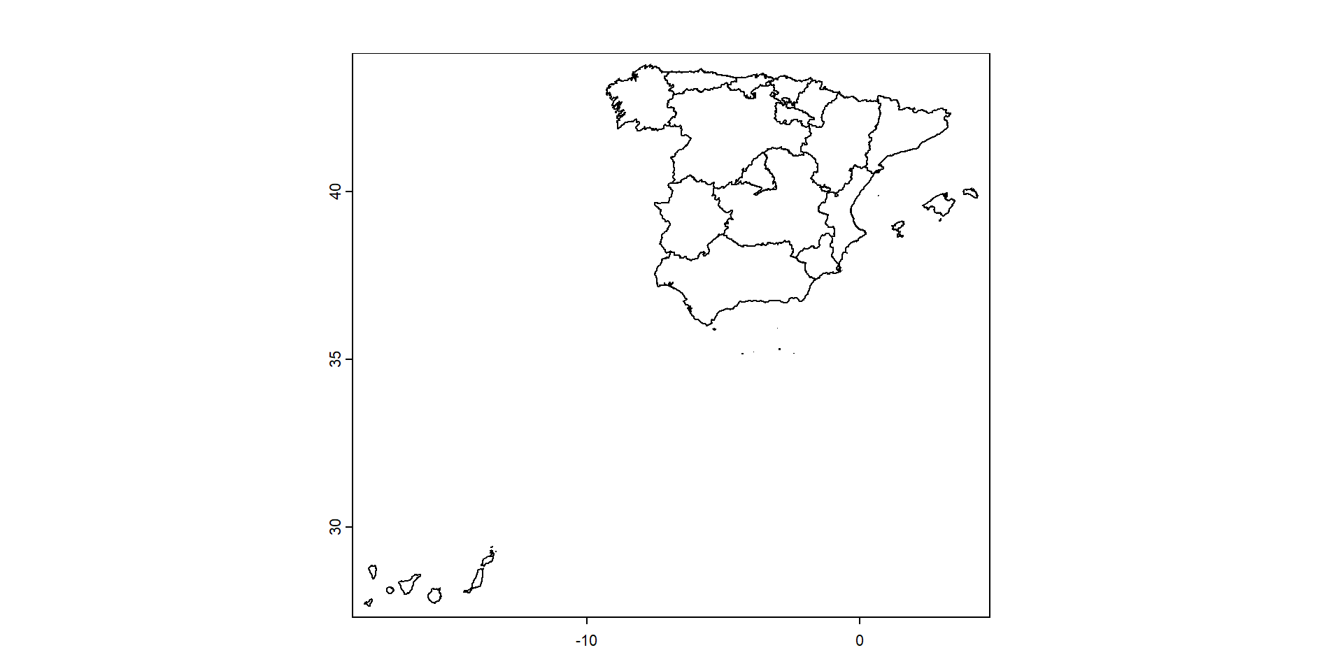
Cambia el CRS pero no las coordenadas en si

par(mfrow = c(1, 4))
plot(esp)
plot(esp_sin_crs)
plot(esp_falso_utm)
plot(esp_false_utm2)

Note

Cambia la representación gráfica porque las unidades cambian entre CRS (grados o metros). Mientras los metros se representan igual en el eje horizontal y vertical, los grados geográficos no.

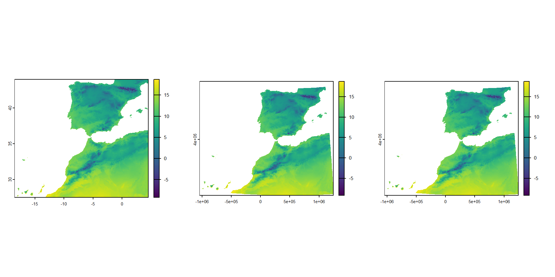
Para convertir coordenadas entre diferentes CRSs tenemos que proyectar los datos

esp_utm30n <- project(esp, "+proj=utm +zone=30 +north +datum=WGS84 +units=m +no_defs +type=crs")
esp_4326 <- project(esp, "EPSG:4326")
par(mfrow = c(1, 3))
plot(esp)
plot(esp_utm30n)
plot(esp_4326)

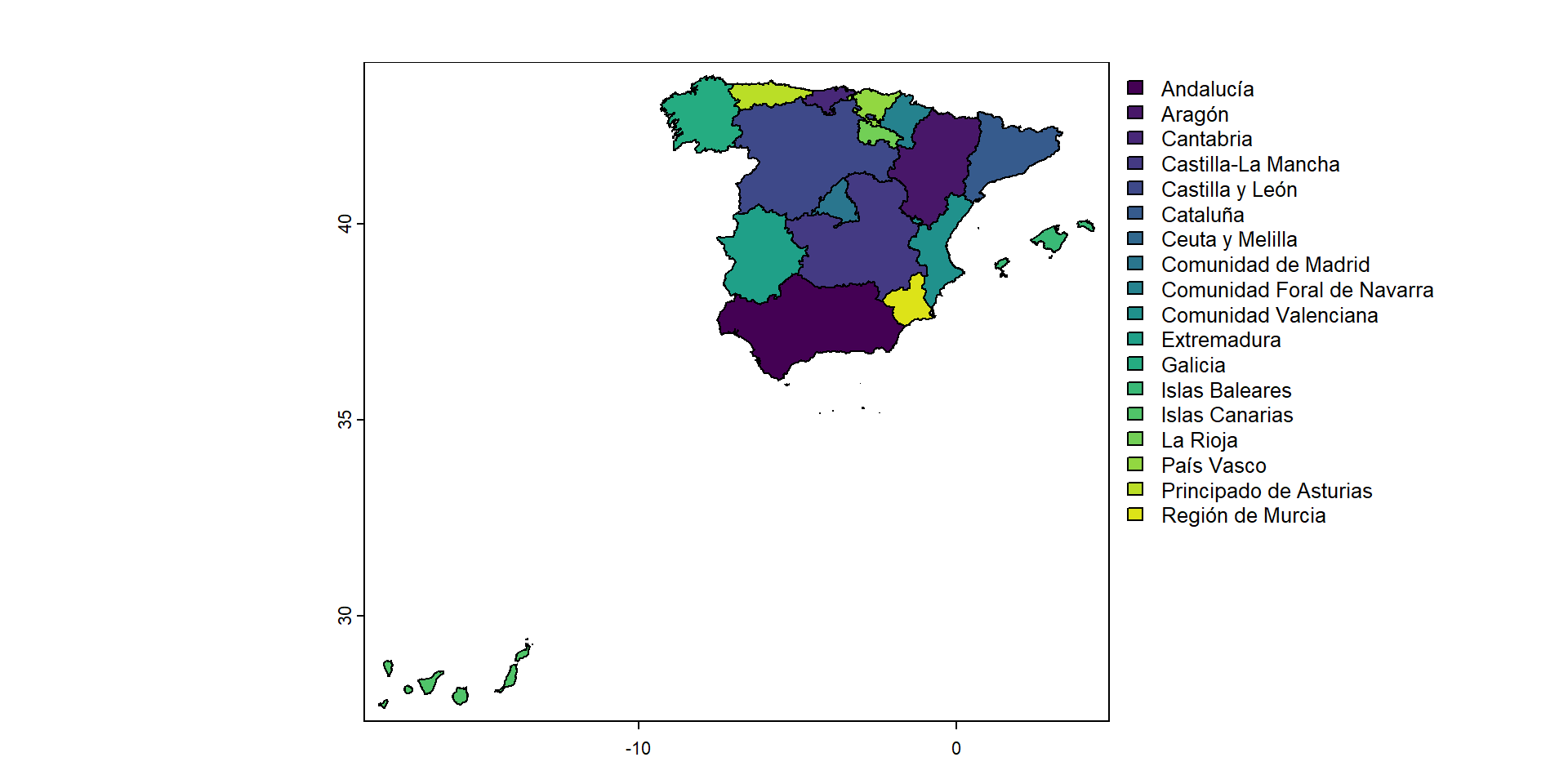
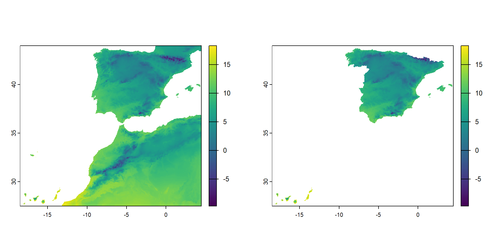
También se puede filtrar la información para una o varias entidades de los datos

which(esp$NAME_1 == "Andalucía")

[1] 1

i <- which(esp$NAME_1 %in% c("Andalucía", "Región de Murcia"))
g <- esp[i,]
plot(g)

Momento para practicar

Ejercicios de clase

Parte 1: Trabajando con datos vectoriales

Manejando datos ráster

Podemos crear datos ráster desde cero

r <- rast(ncol = 10, nrow = 10, 
          xmin = -150, xmax = -80, 
          ymin = 20, ymax = 60)
values(r) <- runif(ncell(r))
r

class       : SpatRaster 
size        : 10, 10, 1  (nrow, ncol, nlyr)
resolution  : 7, 4  (x, y)
extent      : -150, -80, 20, 60  (xmin, xmax, ymin, ymax)
coord. ref. : lon/lat WGS 84 (CRS84) (OGC:CRS84) 
source(s)   : memory
name        :      lyr.1 
min value   : 0.01535991 
max value   : 0.99922492 

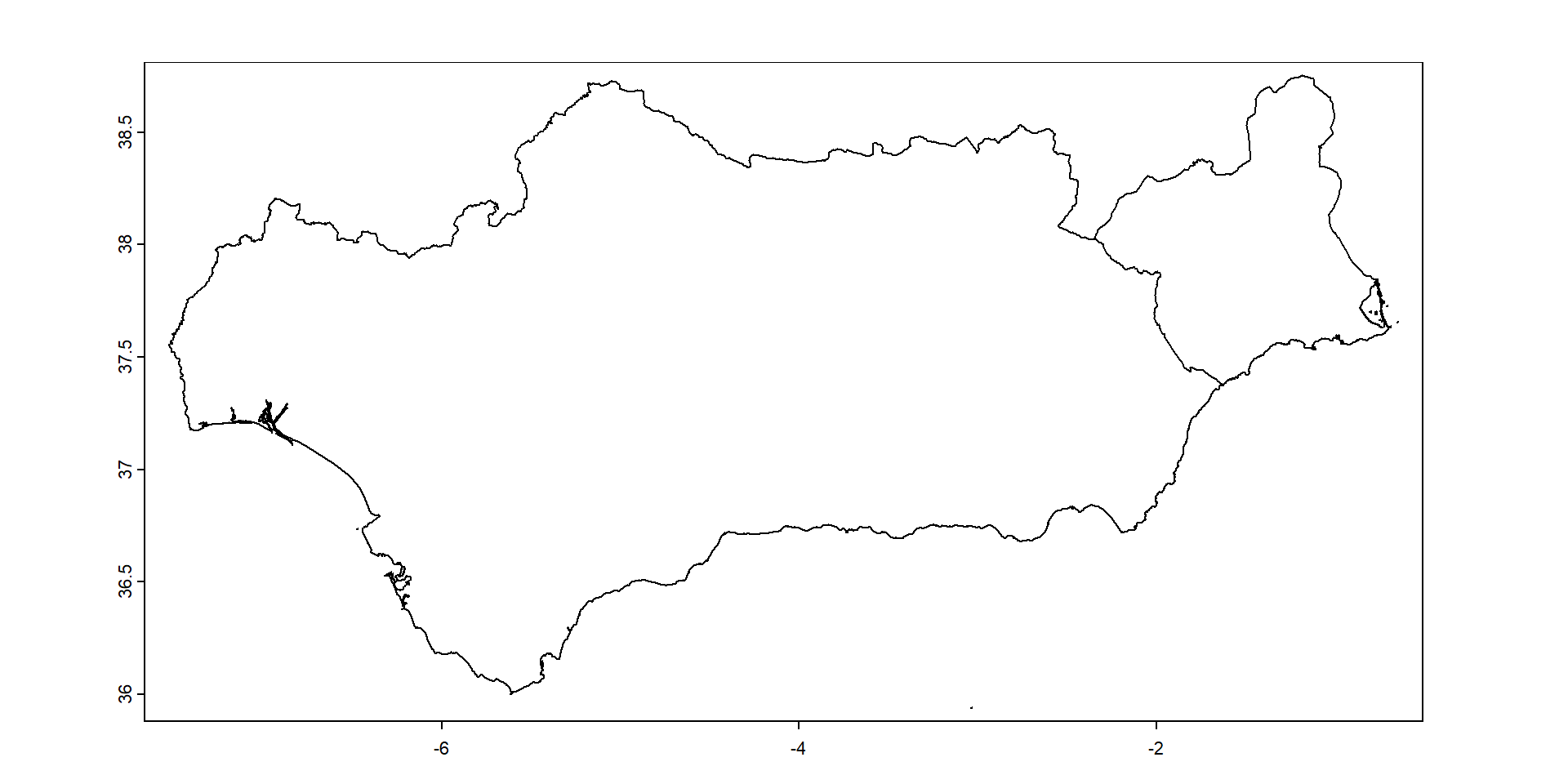
Veamos que aspecto tienen

plot(r)

Podemos operar con los datos ráster

r2 <- r * r
r3  <- sqrt(r)

Important

Al operar con datos ráster, las operaciones se aplican sobre cada píxel individualmente. Por ello, sólo se pueden realizar operaciones con ráster que tienen el mismo área y el mismo tamaño de píxel. El resultado, por tanto, es un nuevo objeto ráster con las mismas características geográficas, pero cuyos píxeles tienen los valores resultantes de aplicar las funciones matemáticas.

Si trabajamos con muchas capas, mejor crear un objeto multicapa

stck <- c(r, r2, r3)
stck

class       : SpatRaster 
size        : 10, 10, 3  (nrow, ncol, nlyr)
resolution  : 7, 4  (x, y)
extent      : -150, -80, 20, 60  (xmin, xmax, ymin, ymax)
coord. ref. : lon/lat WGS 84 (CRS84) (OGC:CRS84) 
source(s)   : memory
names       :      lyr.1,        lyr.1,     lyr.1 
min values  : 0.01535991, 0.0002359268, 0.1239351 
max values  : 0.99922492, 0.9984504488, 0.9996124 

Veamos que aspecto tiene el objeto multicapa

plot(stck)

También se pueden extraer capas de objetos multicapa

r2 <- stck[[2]]
r2

class       : SpatRaster 
size        : 10, 10, 1  (nrow, ncol, nlyr)
resolution  : 7, 4  (x, y)
extent      : -150, -80, 20, 60  (xmin, xmax, ymin, ymax)
coord. ref. : lon/lat WGS 84 (CRS84) (OGC:CRS84) 
source(s)   : memory
name        :        lyr.1 
min value   : 0.0002359268 
max value   : 0.9984504488 

Como antes, lo normal es cargar datos generados en SIG

Para ello podemos descargar datos de distintas fuentes (v.gr. WorldClim)

tavg <- rast("climate/tavg_esp.tif")
tavg

class       : SpatRaster 
size        : 1980, 2760, 12  (nrow, ncol, nlyr)
resolution  : 0.008333333, 0.008333333  (x, y)
extent      : -18.5, 4.5, 27.5, 44  (xmin, xmax, ymin, ymax)
coord. ref. : lon/lat WGS 84 (EPSG:4326) 
source      : tavg_esp.tif 
names       : tavg_esp_1, tavg_esp_2, tavg_esp_3, tavg_esp_4, tavg_esp_5, tavg_esp_6, ... 
min values  :       -9.8,       -9.4,       -7.7,         -6,       -1.4,        3.2, ... 
max values  :       19.2,       18.9,       21.6,         26,       30.4,       36.0, ... 

Como antes, lo normal es cargar datos generados en SIG

… o podemos usar el paquete geodata para acceder directamente a esa información

tavg <- worldclim_country("ESP", "tavg", path = ".")
tavg

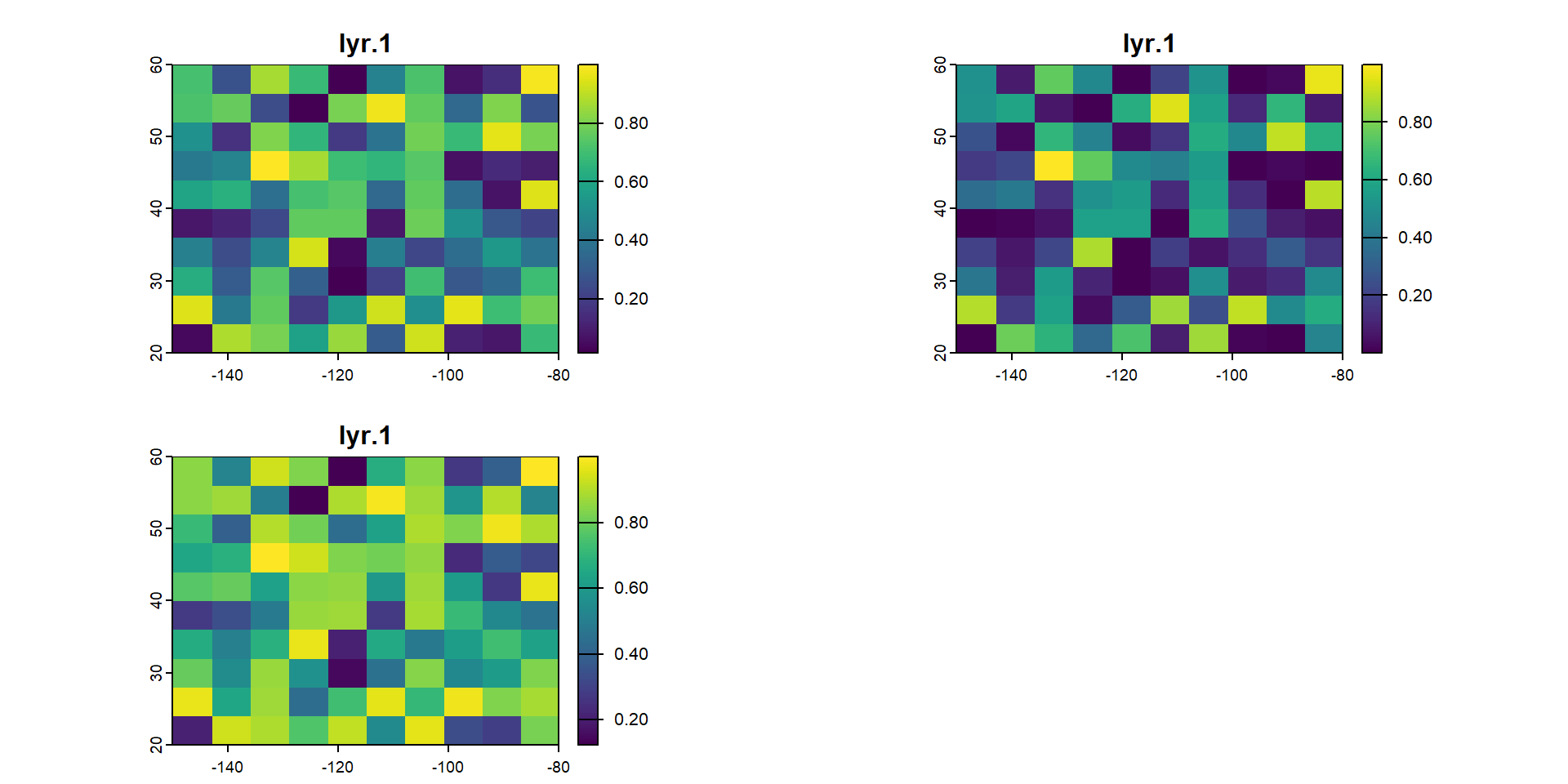
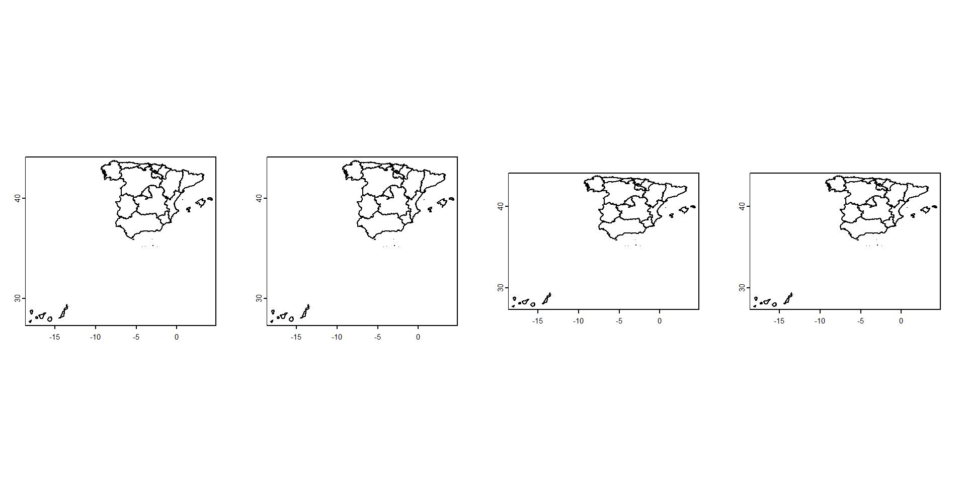
Veamos si se parece a lo que conocemos…

plot(tavg, range = c(-20, 30))

También podemos guardar estos datos para no tener que volver a descargarlos

writeRaster(tavg, "raster_tavg_esp.tif", overwrite = TRUE)

Los datos ráster también se pueden proyectar

tavg_utm30n <- project(tavg, "EPSG:3042")

|---------|---------|---------|---------|
=========================================
                                          

tavg_utm30n

class       : SpatRaster 
size        : 2393, 2805, 12  (nrow, ncol, nlyr)
resolution  : 814.2352, 814.2352  (x, y)
extent      : -1041769, 1242161, 3041688, 4990152  (xmin, xmax, ymin, ymax)
coord. ref. : ETRS89 / UTM zone 30N (N-E) (EPSG:3042) 
source      : spat_6abc64f9a9_27324_o8up7yuDdJ6XHBX.tif 
names       : tavg_esp_1, tavg_esp_2, tavg_esp_3, tavg_esp_4, tavg_esp_5, tavg_esp_6, ... 
min values  :  -9.649184,  -9.150451,  -7.476511,  -5.675769,  -1.142849,   3.455518, ... 
max values  :  19.200001,  18.900000,  21.600000,  26.000000,  30.400000,  36.000000, ... 

Ahora las coordenadas si aparecen “desplazadas”

par(mfrow = c(1, 2))
plot(tavg[[1]])
plot(tavg_utm30n[[1]])

Warning

No hay una correspondencia exacta de píxeles. Lo veréis más claro si revisáis las diapositivas anteriores (39 y 43).

Para controlar el número de pixeles y su resolución podemos crear una “plantilla”

plantilla <- rast(tavg_utm30n)
res(plantilla) <- 800
plantilla

class       : SpatRaster 
size        : 2436, 2855, 12  (nrow, ncol, nlyr)
resolution  : 800, 800  (x, y)
extent      : -1041769, 1242231, 3041688, 4990488  (xmin, xmax, ymin, ymax)
coord. ref. : ETRS89 / UTM zone 30N (N-E) (EPSG:3042) 

tavg_utm30n_plantilla <- project(tavg, plantilla)

|---------|---------|---------|---------|
=========================================
                                          

tavg_utm30n_plantilla

class       : SpatRaster 
size        : 2436, 2855, 12  (nrow, ncol, nlyr)
resolution  : 800, 800  (x, y)
extent      : -1041769, 1242231, 3041688, 4990488  (xmin, xmax, ymin, ymax)
coord. ref. : ETRS89 / UTM zone 30N (N-E) (EPSG:3042) 
source      : spat_6abc5cd96cab_27324_zxzxx9jyyx6UnnI.tif 
names       : tavg_esp_1, tavg_esp_2, tavg_esp_3, tavg_esp_4, tavg_esp_5, tavg_esp_6, ... 
min values  :  -9.669218,  -9.190617,  -7.505003,  -5.726402,  -1.185399,   3.409383, ... 
max values  :  19.200001,  18.900000,  21.600000,  26.000000,  30.400000,  36.000000, ... 

Veamos el resultado

par(mfrow = c(1, 3))
plot(tavg[[2]])
plot(tavg_utm30n[[2]])
plot(tavg_utm30n_plantilla[[2]])

Momento de practicar por vuestra cuenta

Ejercicios de clase

Parte 2. Manejo de datos ráster

Manipular datos espaciales

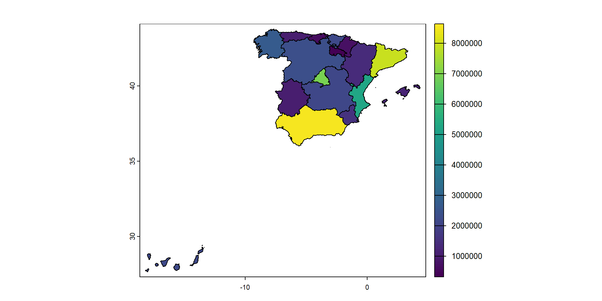
Podemos dibujar los mapas en base a información de los atributos

plot(esp, "NAME_1")

Podemos combinar información ráster y vectorial en el mismo gráfico

plot(tavg[[1]])
plot(esp, add = TRUE)

También se puede extraer información de atributos para trabajar con ella

d <- as.data.frame(esp)
head(d)

    GID_1 GID_0 COUNTRY             NAME_1                        VARNAME_1
1 ESP.1_1   ESP   Spain          Andalucía Andalousie|Andaluc¡a|Andalusien|
2 ESP.2_1   ESP   Spain             Aragón Aragão|Aragó|Aragón|Aragona|Arag
3 ESP.3_1   ESP   Spain          Cantabria Cantàbria|Cantábria|Cantabrie|Ka
4 ESP.4_1   ESP   Spain Castilla-La Mancha Castela-La Mancha|Castela-Mancha
5 ESP.5_1   ESP   Spain    Castilla y León Castile and Leon|Castela e Leão|
6 ESP.6_1   ESP   Spain           Cataluña Catalogna|Catalogne|Catalonia|Ca
  NL_NAME_1             TYPE_1            ENGTYPE_1 CC_1 HASC_1 ISO_1
1      <NA> Comunidad Autónoma Autonomous Community   01  ES.AN  <NA>
2      <NA> Comunidad Autónoma Autonomous Community   15  ES.AR  <NA>
3      <NA> Comunidad Autónoma Autonomous Community   06  ES.CB ES-CB
4      <NA> Comunidad Autónoma Autonomous Community   08  ES.CM ES-CM
5      <NA> Comunidad Autónoma Autonomous Community   07  ES.CL  <NA>
6      <NA> Comunidad Autónoma Autonomous Community   09  ES.CT  <NA>

O puedo extraer la información de uno sólo de los atributos

esp$NAME_1

 [1] "Andalucía"                  "Aragón"                    
 [3] "Cantabria"                  "Castilla-La Mancha"        
 [5] "Castilla y León"            "Cataluña"                  
 [7] "Ceuta y Melilla"            "Comunidad de Madrid"       
 [9] "Comunidad Foral de Navarra" "Comunidad Valenciana"      
[11] "Extremadura"                "Galicia"                   
[13] "Islas Baleares"             "Islas Canarias"            
[15] "La Rioja"                   "País Vasco"                
[17] "Principado de Asturias"     "Región de Murcia"          

esp[, "NAME_1"]

 class       : SpatVector 
 geometry    : polygons 
 dimensions  : 18, 1  (geometries, attributes)
 extent      : -18.16153, 4.328195, 27.63736, 43.79153  (xmin, xmax, ymin, ymax)
 coord. ref. : lon/lat WGS 84 (EPSG:4326) 
 names       :    NAME_1
 type        :     <chr>
 values      : Andalucía
                  Aragón
               Cantabria

Warning

Notad que en este caso, las dos formas de extraer información no se comportan exactamente igual

También podemos extraer las características geográficas (espaciales)

g <- geom(esp_utm30n) 
head(g)

     geom part        x       y hole
[1,]    1    1 497181.4 3977371    0
[2,]    1    1 497181.4 3977340    0
[3,]    1    1 497156.3 3977340    0
[4,]    1    1 497156.3 3977310    0
[5,]    1    1 497106.3 3977310    0
[6,]    1    1 497106.2 3977279    0

Es posible incorporar información a nuestros datos vectoriales

perim(esp)

 [1] 2589087.46 1440885.84  846934.43 2244558.59 2663559.30 1544730.70
 [7]   70829.05  728170.59  729188.20 1504057.15 1326491.81 2511306.43
[13] 1426141.05 1811869.11  553539.59  953048.57  962220.30  778427.60

esp$perimetro <- perim(esp)

expanse(esp)

 [1] 87544528916 47740675073  5309609409 79458825921 94217597811 32110027964
 [7]    29227107  8028465483 10357112866 23260742493 41636776275 29606203571
[13]  5029748466  7510468779  5049234723  7233336501 10602775725 11318963440

esp$area <- expanse(esp)

¿Qué pasa si quiero borrar una columna?

esp$area <- NULL

A veces tenemos los datos en una tabla aparte

Note

Me descargué datos del censo poblacional del país

d <- openxlsx::read.xlsx("data/Censo_poblacional.xlsx",
                         sheet = 1)
d

                    comunidad   total hombres mujeres
1                   Andalucía 8631862 4249355 4382507
2                      Aragón 1351591  668275  683316
3      Principado de Asturias 1009599  481478  528121
4              Islas Baleares 1231768  613910  617858
5              Islas Canarias 2238754 1105037 1133717
6                   Cantabria  590851  286322  304529
7             Castilla y León 2391682 1177504 1214178
8          Castilla-La Mancha 2104433 1055223 1049210
9                    Cataluña 8012231 3943698 4068533
10       Comunidad Valenciana 5319285 2615852 2703433
11                Extremadura 1054681  521677  533004
12                    Galicia 2705833 1301744 1404089
13        Comunidad de Madrid 7009268 3356163 3653105
14           Región de Murcia 1568492  786038  782454
15 Comunidad Foral de Navarra  678333  335919  342414
16                 País Vasco 2227684 1083488 1144196
17                   La Rioja  324184  159979  164205

Podemos vincularla con los datos espaciales

Para vincularla necesitamos un campo en común

esp <- merge(esp, d, 
             by.x = "NAME_1", 
             by.y = "comunidad")
esp

 class       : SpatVector 
 geometry    : polygons 
 dimensions  : 17, 15  (geometries, attributes)
 extent      : -18.16153, 4.328195, 27.63736, 43.79153  (xmin, xmax, ymin, ymax)
 coord. ref. : lon/lat WGS 84 (EPSG:4326) 
 names       :    NAME_1   GID_1 GID_0 COUNTRY       VARNAME_1 NL_NAME_1
 type        :     <chr>   <chr> <chr>   <chr>           <chr>     <chr>
 values      : Andalucía ESP.1_1   ESP   Spain Andalousie|And~        NA
                  Aragón ESP.2_1   ESP   Spain Aragão|Aragó|A~        NA
               Cantabria ESP.3_1   ESP   Spain Cantàbria|Cant~        NA
          TYPE_1       ENGTYPE_1  CC_1 HASC_1 (and 5 more)
           <chr>           <chr> <chr>  <chr>             
 Comunidad Autó~ Autonomous Com~    01  ES.AN             
 Comunidad Autó~ Autonomous Com~    15  ES.AR             
 Comunidad Autó~ Autonomous Com~    06  ES.CB             

Veamos la población Española por provincias

plot(esp, "total", type = "continuous")

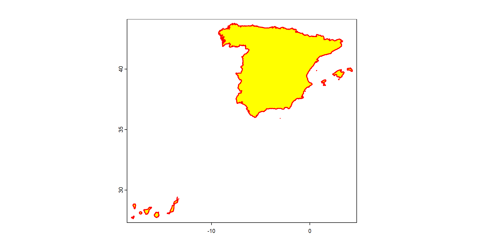
A veces necesitamos fusionar las formas de varios polígonos (o líneas) en uno de mayor tamaño

esp <- aggregate(esp, by = "COUNTRY") 
plot(esp, col = "yellow", lwd = 2, border = "red")

Los objetos ráster también se pueden agregar

Note

La agregación aquí trabaja a nivel de píxel, por lo que se usan para cambiar la resolución de los datos.

tavg_20 <- aggregate(tavg, fact = 20, fun = "mean", na.rm = TRUE)
par(mfrow = c(1, 2))
plot(tavg[[1]])
plot(tavg_20[[1]])

Podemos usar una capa vectorial como máscara para seleccionar objetos dentro de otra capa vectorial

clip <- rast(ext = c(-6, -4, 37, 41), nrow = 2, ncol = 2)
values(clip) <- 1:4
names(clip) <- "Zona"
clip <- as.polygons(clip)
clip 

 class       : SpatVector 
 geometry    : polygons 
 dimensions  : 4, 1  (geometries, attributes)
 extent      : -6, -4, 37, 41  (xmin, xmax, ymin, ymax)
 coord. ref. : lon/lat WGS 84 (CRS84) (OGC:CRS84) 
 names       :  Zona
 type        : <int>
 values      :     1
                   2
                   3

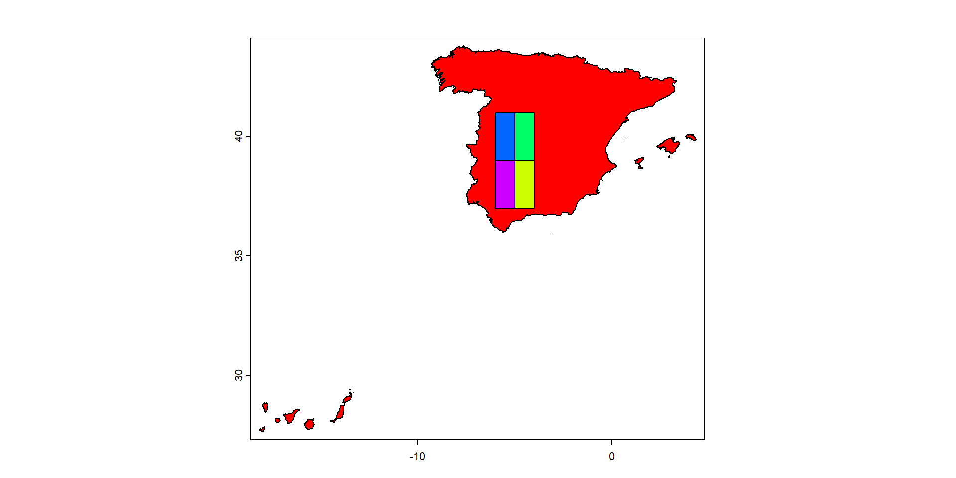
Veamos que aspecto presentan las dos capas

plot(esp) 
plot(clip, add = TRUE, border = "blue", lwd = 5) 

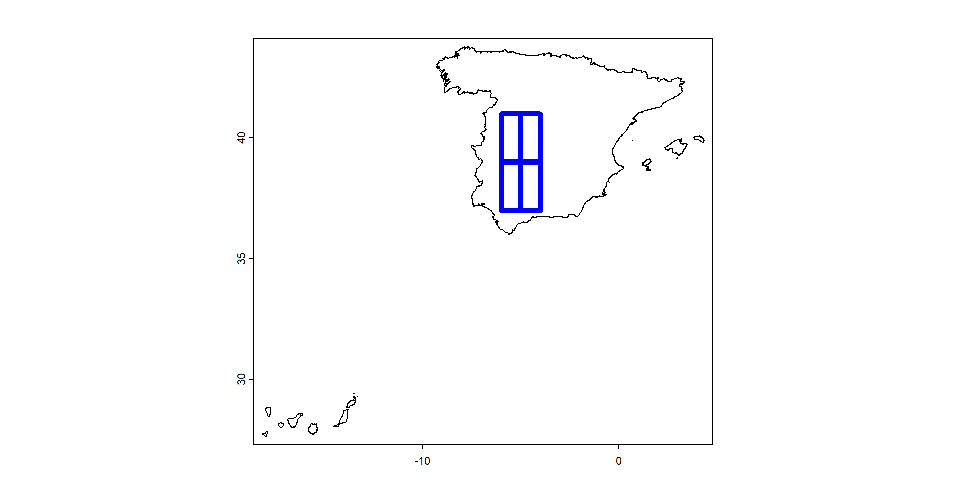
Hagamos la intersección y veamos el resultado

esp_clip <- intersect(esp, clip) 
plot(esp_clip)

Los objetos ráster también se pueden cortar con un vectorial

tavg_esp <- mask(tavg, esp)

|---------|---------|---------|---------|
=========================================
                                          

par(mfrow = c(1, 2))
plot(tavg[[1]])
plot(tavg_esp[[1]])

Otras veces necesitamos combinar las formas de dos objetos vectoriales diferentes

u <- union(esp, clip)
plot(u, col = sample(rainbow(length(u))))

Es muy útil extraer información de una capa vectorial en los puntos, líneas o polígonos de otra capa vectorial

Para ello creamos una capa de puntos cualquiera

pnts <- spatSample(esp, 100)

plot(esp)
plot(clip, add = TRUE, border = "cyan")
plot(pnts, add = TRUE, col = "red")

Veamos los valores de las capas en los puntos

pnts_esp <- extract(esp, pnts)
head(pnts_esp)

  id.y COUNTRY mean_perimetro mean_total mean_hombres mean_mujeres NAME_1 GID_1
1    1   Spain        1447895    2850031      1396568      1453463     NA    NA
2    2   Spain        1447895    2850031      1396568      1453463     NA    NA
3    3   Spain        1447895    2850031      1396568      1453463     NA    NA
4    4   Spain        1447895    2850031      1396568      1453463     NA    NA
5    5   Spain        1447895    2850031      1396568      1453463     NA    NA
6    6   Spain        1447895    2850031      1396568      1453463     NA    NA
  GID_0 VARNAME_1 NL_NAME_1             TYPE_1            ENGTYPE_1 CC_1 HASC_1
1   ESP        NA      <NA> Comunidad Autónoma Autonomous Community   NA     NA
2   ESP        NA      <NA> Comunidad Autónoma Autonomous Community   NA     NA
3   ESP        NA      <NA> Comunidad Autónoma Autonomous Community   NA     NA
4   ESP        NA      <NA> Comunidad Autónoma Autonomous Community   NA     NA
5   ESP        NA      <NA> Comunidad Autónoma Autonomous Community   NA     NA
6   ESP        NA      <NA> Comunidad Autónoma Autonomous Community   NA     NA
  ISO_1 agg_n
1    NA    17
2    NA    17
3    NA    17
4    NA    17
5    NA    17
6    NA    17

pnts_clip <- extract(clip, pnts)
head(pnts_clip)

  id.y Zona
1    1    1
2    2   NA
3    3   NA
4    4   NA
5    5    1
6    6   NA

Igual podemos hacer con respecto a los valores de los píxeles en cada punto de un vectorial

pnts_tavg <- extract(tavg, pnts)
head(pnts_tavg)

  ID tavg_esp_1 tavg_esp_2 tavg_esp_3 tavg_esp_4 tavg_esp_5 tavg_esp_6
1  1        3.6        5.6        7.8        9.7       13.4       17.9
2  2       11.0       12.1       13.9       15.4       18.4       22.2
3  3        3.7        4.9        7.4        9.5       13.7       19.0
4  4        2.2        3.6        6.1        7.5       10.9       15.5
5  5        3.5        5.1        7.3        9.0       12.8       17.5
6  6        5.4        6.3        7.9        9.1       12.5       15.3
  tavg_esp_7 tavg_esp_8 tavg_esp_9 tavg_esp_10 tavg_esp_11 tavg_esp_12
1       21.3       20.9       17.6        12.3         7.6         4.7
2       25.4       25.2       23.0        18.8        14.8        12.1
3       23.2       22.8       18.4        12.6         7.5         4.6
4       18.7       18.4       15.4        10.3         5.9         3.3
5       21.3       20.9       17.5        11.9         7.3         4.5
6       17.8       18.3       16.5        12.9         8.7         6.5

Warning

Fijaros que extrae un valor de cada capa del ráster stack

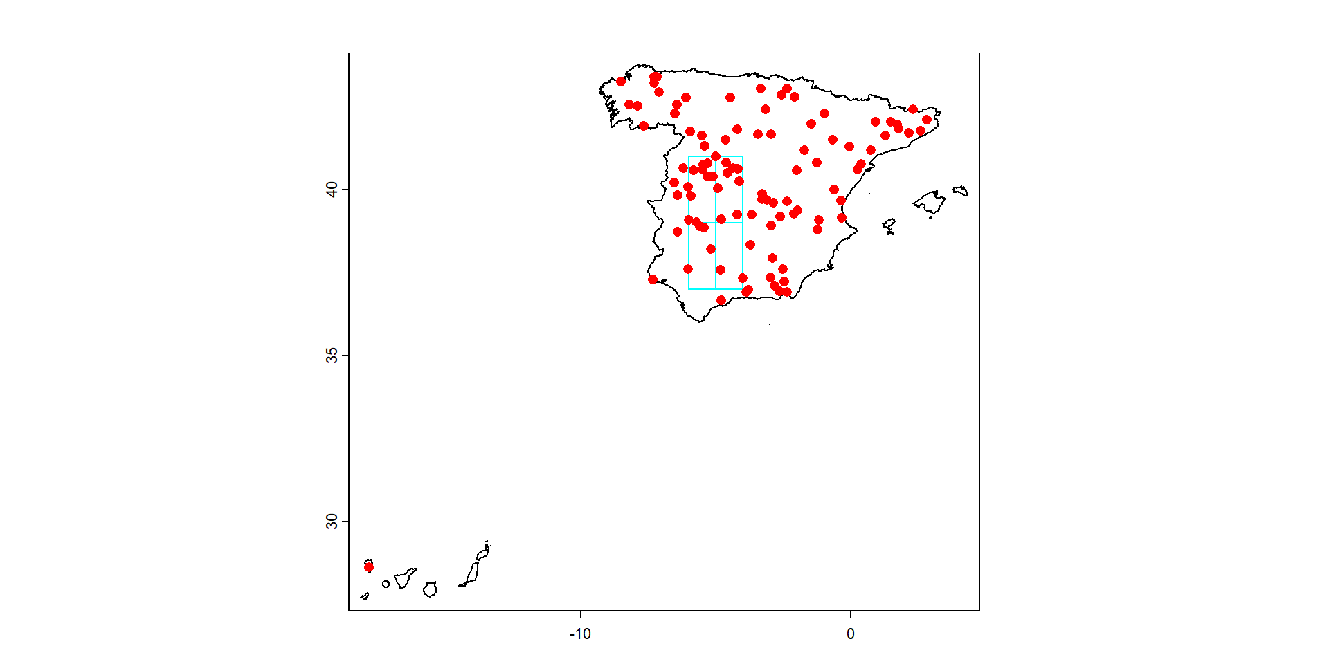
También funciona con polígonos

prov_tavg <- extract(tavg, esp, fun = "mean", bind = TRUE, na.rm = TRUE)
plot(prov_tavg, "tavg_esp_1")

Los objetos ráster se puede operar matemáticamente con ellos para generar estadísticos

min, max, mean, prod, sum, median, cv, range, any y all

min_tavg <- min(tavg)
plot(min_tavg)

También hay multitud de funciones avanzadas propias de un SIG, tanto para vectoriales como ráster

crop, trim, merge, disagg, resample, classify o cover

El paquete gdistance ofrece análisis de distancias complejos (least cost path, etcétera)

Last but not least! Se pueden transformar datos vectoriales en ráster…

esp_raster <- rasterize(esp, tavg, field = "NAME_1")
class(esp_raster)

[1] "SpatRaster"
attr(,"package")
[1] "terra"

plot(esp_raster)

… y viceversa

as.polygons(tavg[[1]])

 class       : SpatVector 
 geometry    : polygons 
 dimensions  : 30, 1  (geometries, attributes)
 extent      : -18.15833, 4.5, 27.5, 44  (xmin, xmax, ymin, ymax)
 coord. ref. : lon/lat WGS 84 (EPSG:4326) 
 names       : tavg_esp_1
 type        :      <int>
 values      :        -10
                       -9
                       -8

Hora de trabajar por vuestra cuenta…

Ejercicios de clase

Parte 3. Manipulación de datos ráster y vectoriales