Modelos Generalizados de Disimilitud en R

Generalized Dissimilarity Models (GDM)

Diego Nieto Lugilde

Universidad de Córdoba (España)

Preparando los datos

Usaremos el paquete gdm. Éste tiene una forma particular de funcionar y especificar los datos. Así que necesitamos prepararlos un poco antes de empezar

library(gdm)

Cargamos los datos de Wilson, incluyendo las coordenadas geográficas

library(openxlsx)
env <- read.xlsx("data/Wilson_Latorre/Data_multi_env_R_course.xlsx", 
                 sheet = 1, 
                 rowNames = TRUE)
com <- read.xlsx("data/Wilson_Latorre/Data_multi_bio_R_course.xlsx", 
                 sheet = 1, 
                 rowNames = TRUE)
coords <- read.xlsx("data/Wilson_Latorre/Data_multi_site_R_course.xlsx", 
                    sheet = 1, 
                    rowNames = TRUE)
summary(coords)

    Sitio              Parcela       Estacion              Año       
 Length:64          Min.   :1.00   Length:64          Min.   :20.00  
 Class :character   1st Qu.:1.75   Class :character   1st Qu.:20.75  
 Mode  :character   Median :2.50   Mode  :character   Median :21.00  
                    Mean   :2.50                      Mean   :21.00  
                    3rd Qu.:3.25                      3rd Qu.:21.25  
                    Max.   :4.00                      Max.   :22.00  
      Long             Lat        
 Min.   :-80.39   Min.   :-1.292  
 1st Qu.:-80.34   1st Qu.:-1.266  
 Median :-80.32   Median :-1.240  
 Mean   :-80.33   Mean   :-1.236  
 3rd Qu.:-80.31   3rd Qu.:-1.211  
 Max.   :-80.29   Max.   :-1.173  

Cargamos los datos bioclimáticos y los incorporamos a las variables ambientales

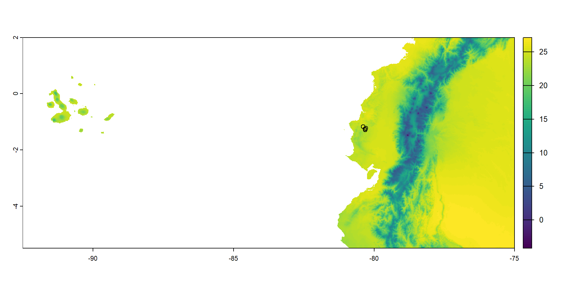
En particular cargamos los datos de Ecuador en formato ráster

Note

Estos datos aprendimos a generarlos durante la clase sobre datos espaciales en R.

library(terra)
library(geodata)
bio <- worldclim_country("ECU", "bio", path = ".")

bio_data <- terra::extract(bio, as.matrix(coords[,c("Long", "Lat")]))
env <- cbind(env, bio_data)

plot(bio[[1]])
points(coords[,c("Long","Lat")])

Reproyectamos los mapas

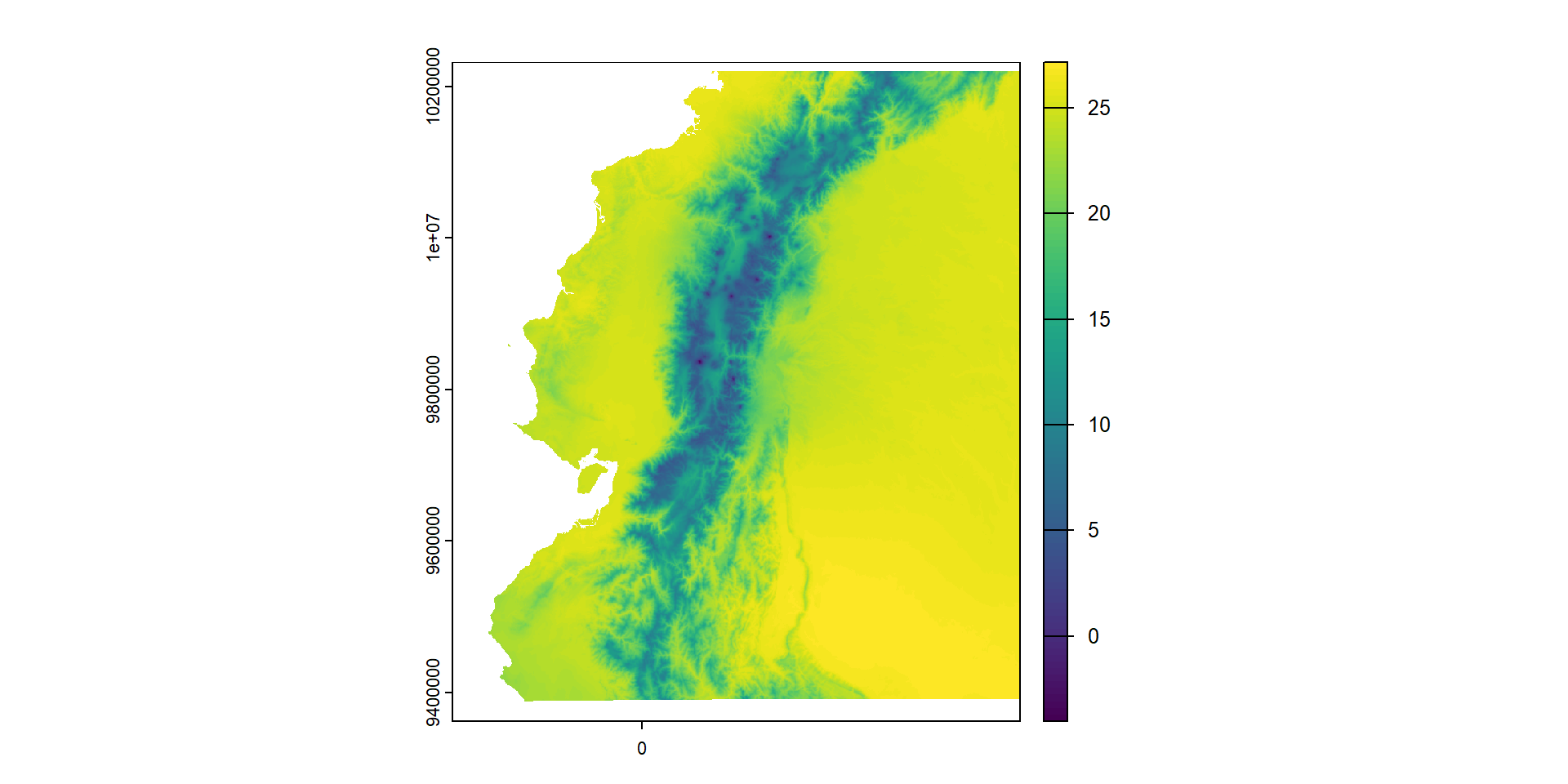
En UTM 18s y los recorto para la región de interés

bio <- project(bio, "EPSG:32718")

|---------|---------|---------|---------|
=========================================
                                          

bio <- crop(bio, 
                ext(-250000, 499746.5, 9362131, 10231857))
plot(bio[[1]])

Reproyecto los datos de coordenadas a UTM 18s y los combino con los datos de comunidades

Important

El paquete gdm requiere que las coordenadas estén especificadas como columnas en la matriz de comunidades, en la matriz de variables ambientales, o en las dos; pero no se pueden especificar como un objeto independiente.

utm <- project(as.matrix(coords[,c("Long", "Lat")]), 
               from = "EPSG: 4326", 
               to = "EPSG:32718")
utm <- data.frame(x = utm[,1], 
                  y = utm[,2],
                    Sitio = rownames(coords))
com$Sitio <- rownames(com)
com <- merge(com, utm, by = "Sitio")
head(com)

     Sitio Acanthagrion Alluaudomyia Anchytarsus Aquarius Axarus Brechmorhoga
1 BA1_SU20           11            0           0        0      0            0
2 BA1_SU21            1            0           0        0      0            0
3 BA1_WI21            0            0           0        0      0            0
4 BA1_WI22            0            0           0        0      0            0
5 BA2_SU20            6            0           0        0      0            0
6 BA2_SU21            0            0           0        0      0            0
  Buenoa Charmatometra Cylloepus Erythemis Eurygerris Halobatopsis Hebrus
1     50             0         0         0          0            0      0
2      0             0         0         0          1            0      0
3      0             0         0         0          2            1      0
4      0             0         0         0          0            0      0
5     19             0         0         0          0            0      0
6      0             0         1         0          4            0     10
  Helochares Hetaerina Heterelmis Hexatoma Husseyella Hydrometra Hydroscapha
1          0         1          0        0          0          0           0
2          0         2          0        0         22          0           0
3          0         0          0        0         19          0           0
4          0         0          0        0         12          0           0
5          0         3          0        0          0          0           0
6          0         0          1        0          6          0           0
  Laccodytes Leptohyphes Leptonema Limnocoris Limnogonus Macrogynoplax
1         46           1         1          3          0             1
2         28           0         0          2          2             0
3         13           8         0          0          0             0
4          0           0         0          0          0             0
5         70           0         1          3          0             0
6         79           1         0          0          1             0
  Macrothemis Mesovelia Microvelia Paracloeodes Pelocoris Phyllogomphoides
1           0         0          0            0         5                4
2           0         0          6            0         2                1
3           0         0          7            0         0                0
4           0         0          0            0         0                0
5           0         0          0            0         1                0
6           0         2          0            0         0                0
  Phylloicus Rhagovelia Scirtes Simulium Stridulivelia Telmatometra
1         11         32       0        0             0            0
2          3         63       1        0            73            0
3          7         33       0        0             0            0
4          0          7       0        0             0            0
5          9          0       0        0             0            0
6          5         16       0        0            10            0
  Telmatometroides Thraulodes Tipula Tricorythodes Melanoides Lymnaea Pomacea
1                0         26      0             1          0       0       0
2                0          6      0             2          0       0       0
3                0          3      0             2          0       0       0
4                0          0      0             0          0       0       0
5                0         56      0             5          0       0       0
6                0          7      0             0          0       0       0
  Pseudothelphusidae Hyalella         x       y
1                  0        0 -91852.58 9856630
2                  0        0 -91852.58 9856630
3                  0        0 -91852.58 9856630
4                  0        0 -91852.58 9856630
5                  3        0 -91852.58 9856630
6                  0        0 -91852.58 9856630

Genero un identificador de sitio común para la matriz de comunidades y la de variables ambientales

com$site_id <- as.numeric(1:nrow(com))
env$site_id <- as.numeric(1:nrow(com))
head(env)

         N-NO3- N-NH3 N-NO2- PO43-    pH    DO    EC   NTU    T°C
SC1_SU20   0.02  0.09  0.003  1.20 9.165 1.840 489.0  8.10 22.180
SC2_SU20   0.02  0.10  0.003  1.12 9.230 1.860 489.0  8.55 22.495
SC3_SU20   0.02  0.13  0.005  3.86 9.115 1.905 472.0  7.70 23.035
SC4_SU20   0.02  0.18  0.003  4.09 8.745 1.985 483.5  8.15 22.445
BA1_SU20   0.05  0.03  0.006  0.73 8.200 5.950 441.5 11.40 19.300
BA2_SU20   0.04  0.10  0.005  0.72 8.940 5.950 166.5 11.85 19.945
         Current.velocity Average.depth Average.width wc2.1_30s_bio_1
SC1_SU20        0.3454020         0.055         0.300        23.84583
SC2_SU20        0.1731571         0.055         0.400        23.84583
SC3_SU20        0.1848344         0.050         0.825        23.84583
SC4_SU20        0.4827096         0.025         0.130        23.84583
BA1_SU20        0.2882227         0.065         0.140        23.89167
BA2_SU20        0.2490695         0.025         0.255        23.89167
         wc2.1_30s_bio_2 wc2.1_30s_bio_3 wc2.1_30s_bio_4 wc2.1_30s_bio_5
SC1_SU20        9.391666        76.98088        91.21548            29.8
SC2_SU20        9.391666        76.98088        91.21548            29.8
SC3_SU20        9.391666        76.98088        91.21548            29.8
SC4_SU20        9.391666        76.98088        91.21548            29.8
BA1_SU20        9.466667        76.34409       101.59706            29.9
BA2_SU20        9.466667        76.34409       101.59706            29.9
         wc2.1_30s_bio_6 wc2.1_30s_bio_7 wc2.1_30s_bio_8 wc2.1_30s_bio_9
SC1_SU20            17.6            12.2        24.85000        22.93333
SC2_SU20            17.6            12.2        24.85000        22.93333
SC3_SU20            17.6            12.2        24.85000        22.93333
SC4_SU20            17.6            12.2        24.85000        22.93333
BA1_SU20            17.5            12.4        25.18333        22.85000
BA2_SU20            17.5            12.4        25.18333        22.85000
         wc2.1_30s_bio_10 wc2.1_30s_bio_11 wc2.1_30s_bio_12 wc2.1_30s_bio_13
SC1_SU20         25.01667         22.83333             1079              279
SC2_SU20         25.01667         22.83333             1079              279
SC3_SU20         25.01667         22.83333             1079              279
SC4_SU20         25.01667         22.83333             1079              279
BA1_SU20         25.18333         22.73333             1119              291
BA2_SU20         25.18333         22.73333             1119              291
         wc2.1_30s_bio_14 wc2.1_30s_bio_15 wc2.1_30s_bio_16 wc2.1_30s_bio_17
SC1_SU20                6         108.9202              685               22
SC2_SU20                6         108.9202              685               22
SC3_SU20                6         108.9202              685               22
SC4_SU20                6         108.9202              685               22
BA1_SU20                5         108.7879              705               22
BA2_SU20                5         108.7879              705               22
         wc2.1_30s_bio_18 wc2.1_30s_bio_19 site_id
SC1_SU20              682               25       1
SC2_SU20              682               25       2
SC3_SU20              682               25       3
SC4_SU20              682               25       4
BA1_SU20              705               25       5
BA2_SU20              705               25       6

Calibrando modelos GDM

Usamos el paquete gdm

Creamos la tabla de disimilaridades

library(gdm)
gdmTab <- formatsitepair(com[,-1], # Quito la columna `Sitio`
               bioFormat = 1, 
               abundance = TRUE, 
               XColumn = "x", # Nombre de la coordenada X
               YColumn = "y", # Nombre de la coordenada Y
               siteColumn = "site_id", # Nombre del identificador
               predData = env) # Quito columnas de texto

gdmRast <- formatsitepair(com[,-1],
               bioFormat = 1, 
               abundance = TRUE, 
               XColumn = "x",
               YColumn = "y", 
               siteColumn = "site_id",
               predData = bio)

head(gdmTab)

            distance weights s1.xCoord s1.yCoord s2.xCoord s2.yCoord s1.N-NO3-
SC1_SU20   0.6225490       1 -91852.58   9856630 -91852.58   9856630      0.02
SC1_SU20.1 0.6041667       1 -91852.58   9856630 -91852.58   9856630      0.02
SC1_SU20.2 0.9339623       1 -91852.58   9856630 -91852.58   9856630      0.02
SC1_SU20.3 0.3875339       1 -91852.58   9856630 -91852.58   9856630      0.02
SC1_SU20.4 0.5535714       1 -91852.58   9856630 -91852.58   9856630      0.02
SC1_SU20.5 0.7301038       1 -91852.58   9856630 -91852.58   9856630      0.02
           s1.N-NH3 s1.N-NO2- s1.PO43- s1.pH s1.DO s1.EC s1.NTU s1.T°C
SC1_SU20       0.09     0.003      1.2 9.165  1.84   489    8.1  22.18
SC1_SU20.1     0.09     0.003      1.2 9.165  1.84   489    8.1  22.18
SC1_SU20.2     0.09     0.003      1.2 9.165  1.84   489    8.1  22.18
SC1_SU20.3     0.09     0.003      1.2 9.165  1.84   489    8.1  22.18
SC1_SU20.4     0.09     0.003      1.2 9.165  1.84   489    8.1  22.18
SC1_SU20.5     0.09     0.003      1.2 9.165  1.84   489    8.1  22.18
           s1.Current.velocity s1.Average.depth s1.Average.width
SC1_SU20              0.345402            0.055              0.3
SC1_SU20.1            0.345402            0.055              0.3
SC1_SU20.2            0.345402            0.055              0.3
SC1_SU20.3            0.345402            0.055              0.3
SC1_SU20.4            0.345402            0.055              0.3
SC1_SU20.5            0.345402            0.055              0.3
           s1.wc2.1_30s_bio_1 s1.wc2.1_30s_bio_2 s1.wc2.1_30s_bio_3
SC1_SU20             23.84583           9.391666           76.98088
SC1_SU20.1           23.84583           9.391666           76.98088
SC1_SU20.2           23.84583           9.391666           76.98088
SC1_SU20.3           23.84583           9.391666           76.98088
SC1_SU20.4           23.84583           9.391666           76.98088
SC1_SU20.5           23.84583           9.391666           76.98088
           s1.wc2.1_30s_bio_4 s1.wc2.1_30s_bio_5 s1.wc2.1_30s_bio_6
SC1_SU20             91.21548               29.8               17.6
SC1_SU20.1           91.21548               29.8               17.6
SC1_SU20.2           91.21548               29.8               17.6
SC1_SU20.3           91.21548               29.8               17.6
SC1_SU20.4           91.21548               29.8               17.6
SC1_SU20.5           91.21548               29.8               17.6
           s1.wc2.1_30s_bio_7 s1.wc2.1_30s_bio_8 s1.wc2.1_30s_bio_9
SC1_SU20                 12.2              24.85           22.93333
SC1_SU20.1               12.2              24.85           22.93333
SC1_SU20.2               12.2              24.85           22.93333
SC1_SU20.3               12.2              24.85           22.93333
SC1_SU20.4               12.2              24.85           22.93333
SC1_SU20.5               12.2              24.85           22.93333
           s1.wc2.1_30s_bio_10 s1.wc2.1_30s_bio_11 s1.wc2.1_30s_bio_12
SC1_SU20              25.01667            22.83333                1079
SC1_SU20.1            25.01667            22.83333                1079
SC1_SU20.2            25.01667            22.83333                1079
SC1_SU20.3            25.01667            22.83333                1079
SC1_SU20.4            25.01667            22.83333                1079
SC1_SU20.5            25.01667            22.83333                1079
           s1.wc2.1_30s_bio_13 s1.wc2.1_30s_bio_14 s1.wc2.1_30s_bio_15
SC1_SU20                   279                   6            108.9202
SC1_SU20.1                 279                   6            108.9202
SC1_SU20.2                 279                   6            108.9202
SC1_SU20.3                 279                   6            108.9202
SC1_SU20.4                 279                   6            108.9202
SC1_SU20.5                 279                   6            108.9202
           s1.wc2.1_30s_bio_16 s1.wc2.1_30s_bio_17 s1.wc2.1_30s_bio_18
SC1_SU20                   685                  22                 682
SC1_SU20.1                 685                  22                 682
SC1_SU20.2                 685                  22                 682
SC1_SU20.3                 685                  22                 682
SC1_SU20.4                 685                  22                 682
SC1_SU20.5                 685                  22                 682
           s1.wc2.1_30s_bio_19 s2.N-NO3- s2.N-NH3 s2.N-NO2- s2.PO43- s2.pH
SC1_SU20                    25      0.02     0.10     0.003     1.12 9.230
SC1_SU20.1                  25      0.02     0.13     0.005     3.86 9.115
SC1_SU20.2                  25      0.02     0.18     0.003     4.09 8.745
SC1_SU20.3                  25      0.05     0.03     0.006     0.73 8.200
SC1_SU20.4                  25      0.04     0.10     0.005     0.72 8.940
SC1_SU20.5                  25      0.05     0.09     0.004     0.57 8.895
           s2.DO s2.EC s2.NTU s2.T°C s2.Current.velocity s2.Average.depth
SC1_SU20   1.860 489.0   8.55 22.495           0.1731571           0.0550
SC1_SU20.1 1.905 472.0   7.70 23.035           0.1848344           0.0500
SC1_SU20.2 1.985 483.5   8.15 22.445           0.4827096           0.0250
SC1_SU20.3 5.950 441.5  11.40 19.300           0.2882227           0.0650
SC1_SU20.4 5.950 166.5  11.85 19.945           0.2490695           0.0250
SC1_SU20.5 5.865 164.0  23.50 19.965           0.1663898           0.0225
           s2.Average.width s2.wc2.1_30s_bio_1 s2.wc2.1_30s_bio_2
SC1_SU20              0.400           23.84583           9.391666
SC1_SU20.1            0.825           23.84583           9.391666
SC1_SU20.2            0.130           23.84583           9.391666
SC1_SU20.3            0.140           23.89167           9.466667
SC1_SU20.4            0.255           23.89167           9.466667
SC1_SU20.5            0.160           23.89167           9.466667
           s2.wc2.1_30s_bio_3 s2.wc2.1_30s_bio_4 s2.wc2.1_30s_bio_5
SC1_SU20             76.98088           91.21548               29.8
SC1_SU20.1           76.98088           91.21548               29.8
SC1_SU20.2           76.98088           91.21548               29.8
SC1_SU20.3           76.34409          101.59706               29.9
SC1_SU20.4           76.34409          101.59706               29.9
SC1_SU20.5           76.34409          101.59706               29.9
           s2.wc2.1_30s_bio_6 s2.wc2.1_30s_bio_7 s2.wc2.1_30s_bio_8
SC1_SU20                 17.6               12.2           24.85000
SC1_SU20.1               17.6               12.2           24.85000
SC1_SU20.2               17.6               12.2           24.85000
SC1_SU20.3               17.5               12.4           25.18333
SC1_SU20.4               17.5               12.4           25.18333
SC1_SU20.5               17.5               12.4           25.18333
           s2.wc2.1_30s_bio_9 s2.wc2.1_30s_bio_10 s2.wc2.1_30s_bio_11
SC1_SU20             22.93333            25.01667            22.83333
SC1_SU20.1           22.93333            25.01667            22.83333
SC1_SU20.2           22.93333            25.01667            22.83333
SC1_SU20.3           22.85000            25.18333            22.73333
SC1_SU20.4           22.85000            25.18333            22.73333
SC1_SU20.5           22.85000            25.18333            22.73333
           s2.wc2.1_30s_bio_12 s2.wc2.1_30s_bio_13 s2.wc2.1_30s_bio_14
SC1_SU20                  1079                 279                   6
SC1_SU20.1                1079                 279                   6
SC1_SU20.2                1079                 279                   6
SC1_SU20.3                1119                 291                   5
SC1_SU20.4                1119                 291                   5
SC1_SU20.5                1119                 291                   5
           s2.wc2.1_30s_bio_15 s2.wc2.1_30s_bio_16 s2.wc2.1_30s_bio_17
SC1_SU20              108.9202                 685                  22
SC1_SU20.1            108.9202                 685                  22
SC1_SU20.2            108.9202                 685                  22
SC1_SU20.3            108.7879                 705                  22
SC1_SU20.4            108.7879                 705                  22
SC1_SU20.5            108.7879                 705                  22
           s2.wc2.1_30s_bio_18 s2.wc2.1_30s_bio_19
SC1_SU20                   682                  25
SC1_SU20.1                 682                  25
SC1_SU20.2                 682                  25
SC1_SU20.3                 705                  25
SC1_SU20.4                 705                  25
SC1_SU20.5                 705                  25

Calibramos los modelos

# Activo que incluya la distancia geográfica en el análisis
gdmTab.fit <- gdm(data=gdmTab, geo=TRUE)
gdmRast.fit <- gdm(data=gdmRast, geo=TRUE)

Analicemos los resultados

Veamos los resultados de los datos de Wilson

summary(gdmTab.fit)

[1] 
[1] 
[1] GDM Modelling Summary
[1] Creation Date:  Thu Oct  9 13:50:52 2025
[1] 
[1] Name:  gdmTab.fit
[1] 
[1] Data:  gdmTab
[1] 
[1] Samples:  2016
[1] 
[1] Geographical distance used in model fitting?  TRUE
[1] 
[1] NULL Deviance:  399.729
[1] GDM Deviance:  335.395
[1] Percent Deviance Explained:  16.094
[1] 
[1] Intercept:  0.848
[1] 
[1] PREDICTOR ORDER BY SUM OF I-SPLINE COEFFICIENTS:
[1] 
[1] Predictor 1: T°C
[1] Splines: 3
[1] Min Knot: 19.3
[1] 50% Knot: 21.502
[1] Max Knot: 23.32
[1] Coefficient[1]: 0.625
[1] Coefficient[2]: 0
[1] Coefficient[3]: 0
[1] Sum of coefficients for T°C: 0.625
[1] 
[1] Predictor 2: Geographic
[1] Splines: 3
[1] Min Knot: 0
[1] 50% Knot: 7872.39
[1] Max Knot: 15526.336
[1] Coefficient[1]: 0.446
[1] Coefficient[2]: 0
[1] Coefficient[3]: 0
[1] Sum of coefficients for Geographic: 0.446
[1] 
[1] Predictor 3: DO
[1] Splines: 3
[1] Min Knot: 1.68
[1] 50% Knot: 5.578
[1] Max Knot: 7.785
[1] Coefficient[1]: 0.32
[1] Coefficient[2]: 0
[1] Coefficient[3]: 0
[1] Sum of coefficients for DO: 0.32
[1] 
[1] Predictor 4: PO43-
[1] Splines: 3
[1] Min Knot: 0.16
[1] 50% Knot: 0.67
[1] Max Knot: 4.09
[1] Coefficient[1]: 0.264
[1] Coefficient[2]: 0
[1] Coefficient[3]: 0
[1] Sum of coefficients for PO43-: 0.264
[1] 
[1] Predictor 5: N-NO3-
[1] Splines: 3
[1] Min Knot: 0.01
[1] 50% Knot: 0.05
[1] Max Knot: 0.39
[1] Coefficient[1]: 0
[1] Coefficient[2]: 0
[1] Coefficient[3]: 0.153
[1] Sum of coefficients for N-NO3-: 0.153
[1] 
[1] Predictor 6: N-NO2-
[1] Splines: 3
[1] Min Knot: 0.001
[1] 50% Knot: 0.005
[1] Max Knot: 0.017
[1] Coefficient[1]: 0.152
[1] Coefficient[2]: 0
[1] Coefficient[3]: 0
[1] Sum of coefficients for N-NO2-: 0.152
[1] 
[1] Predictor 7: NTU
[1] Splines: 3
[1] Min Knot: 2.75
[1] 50% Knot: 14.9
[1] Max Knot: 128.5
[1] Coefficient[1]: 0
[1] Coefficient[2]: 0
[1] Coefficient[3]: 0.141
[1] Sum of coefficients for NTU: 0.141
[1] 
[1] Predictor 8: N-NH3
[1] Splines: 3
[1] Min Knot: 0.008
[1] 50% Knot: 0.1
[1] Max Knot: 0.18
[1] Coefficient[1]: 0
[1] Coefficient[2]: 0
[1] Coefficient[3]: 0
[1] Sum of coefficients for N-NH3: 0
[1] 
[1] Predictor 9: pH
[1] Splines: 3
[1] Min Knot: 7.33
[1] 50% Knot: 8.265
[1] Max Knot: 9.23
[1] Coefficient[1]: 0
[1] Coefficient[2]: 0
[1] Coefficient[3]: 0
[1] Sum of coefficients for pH: 0
[1] 
[1] Predictor 10: EC
[1] Splines: 3
[1] Min Knot: 117
[1] 50% Knot: 394.25
[1] Max Knot: 1641
[1] Coefficient[1]: 0
[1] Coefficient[2]: 0
[1] Coefficient[3]: 0
[1] Sum of coefficients for EC: 0
[1] 
[1] Predictor 11: Current.velocity
[1] Splines: 3
[1] Min Knot: 0.117
[1] 50% Knot: 0.425
[1] Max Knot: 76.452
[1] Coefficient[1]: 0
[1] Coefficient[2]: 0
[1] Coefficient[3]: 0
[1] Sum of coefficients for Current.velocity: 0
[1] 
[1] Predictor 12: Average.depth
[1] Splines: 3
[1] Min Knot: 0.007
[1] 50% Knot: 0.038
[1] Max Knot: 0.155
[1] Coefficient[1]: 0
[1] Coefficient[2]: 0
[1] Coefficient[3]: 0
[1] Sum of coefficients for Average.depth: 0
[1] 
[1] Predictor 13: Average.width
[1] Splines: 3
[1] Min Knot: 0.13
[1] 50% Knot: 0.51
[1] Max Knot: 4.75
[1] Coefficient[1]: 0
[1] Coefficient[2]: 0
[1] Coefficient[3]: 0
[1] Sum of coefficients for Average.width: 0
[1] 
[1] Predictor 14: wc2.1_30s_bio_1
[1] Splines: 3
[1] Min Knot: 23.846
[1] 50% Knot: 24.129
[1] Max Knot: 25.142
[1] Coefficient[1]: 0
[1] Coefficient[2]: 0
[1] Coefficient[3]: 0
[1] Sum of coefficients for wc2.1_30s_bio_1: 0
[1] 
[1] Predictor 15: wc2.1_30s_bio_2
[1] Splines: 3
[1] Min Knot: 9.392
[1] 50% Knot: 9.55
[1] Max Knot: 10.067
[1] Coefficient[1]: 0
[1] Coefficient[2]: 0
[1] Coefficient[3]: 0
[1] Sum of coefficients for wc2.1_30s_bio_2: 0
[1] 
[1] Predictor 16: wc2.1_30s_bio_3
[1] Splines: 3
[1] Min Knot: 76.344
[1] 50% Knot: 77.024
[1] Max Knot: 80.533
[1] Coefficient[1]: 0
[1] Coefficient[2]: 0
[1] Coefficient[3]: 0
[1] Sum of coefficients for wc2.1_30s_bio_3: 0
[1] 
[1] Predictor 17: wc2.1_30s_bio_4
[1] Splines: 3
[1] Min Knot: 77.777
[1] 50% Knot: 93.404
[1] Max Knot: 101.597
[1] Coefficient[1]: 0
[1] Coefficient[2]: 0
[1] Coefficient[3]: 0
[1] Sum of coefficients for wc2.1_30s_bio_4: 0
[1] 
[1] Predictor 18: wc2.1_30s_bio_5
[1] Splines: 3
[1] Min Knot: 29.8
[1] 50% Knot: 30.2
[1] Max Knot: 31.2
[1] Coefficient[1]: 0
[1] Coefficient[2]: 0
[1] Coefficient[3]: 0
[1] Sum of coefficients for wc2.1_30s_bio_5: 0
[1] 
[1] Predictor 19: wc2.1_30s_bio_6
[1] Splines: 3
[1] Min Knot: 17.5
[1] 50% Knot: 17.8
[1] Max Knot: 18.7
[1] Coefficient[1]: 0
[1] Coefficient[2]: 0
[1] Coefficient[3]: 0
[1] Sum of coefficients for wc2.1_30s_bio_6: 0
[1] 
[1] Predictor 20: wc2.1_30s_bio_7
[1] Splines: 3
[1] Min Knot: 12.2
[1] 50% Knot: 12.45
[1] Max Knot: 12.5
[1] Coefficient[1]: 0
[1] Coefficient[2]: 0
[1] Coefficient[3]: 0
[1] Sum of coefficients for wc2.1_30s_bio_7: 0
[1] 
[1] Predictor 21: wc2.1_30s_bio_8
[1] Splines: 3
[1] Min Knot: 24.85
[1] 50% Knot: 25.317
[1] Max Knot: 26.017
[1] Coefficient[1]: 0
[1] Coefficient[2]: 0
[1] Coefficient[3]: 0
[1] Sum of coefficients for wc2.1_30s_bio_8: 0
[1] 
[1] Predictor 22: wc2.1_30s_bio_9
[1] Splines: 3
[1] Min Knot: 22.85
[1] 50% Knot: 23.158
[1] Max Knot: 24.317
[1] Coefficient[1]: 0
[1] Coefficient[2]: 0
[1] Coefficient[3]: 0
[1] Sum of coefficients for wc2.1_30s_bio_9: 0
[1] 
[1] Predictor 23: wc2.1_30s_bio_10
[1] Splines: 3
[1] Min Knot: 25.017
[1] 50% Knot: 25.4
[1] Max Knot: 26.15
[1] Coefficient[1]: 0
[1] Coefficient[2]: 0
[1] Coefficient[3]: 0
[1] Sum of coefficients for wc2.1_30s_bio_10: 0
[1] 
[1] Predictor 24: wc2.1_30s_bio_11
[1] Splines: 3
[1] Min Knot: 22.733
[1] 50% Knot: 23.067
[1] Max Knot: 24.3
[1] Coefficient[1]: 0
[1] Coefficient[2]: 0
[1] Coefficient[3]: 0
[1] Sum of coefficients for wc2.1_30s_bio_11: 0
[1] 
[1] Predictor 25: wc2.1_30s_bio_12
[1] Splines: 3
[1] Min Knot: 729
[1] 50% Knot: 1047.5
[1] Max Knot: 1119
[1] Coefficient[1]: 0
[1] Coefficient[2]: 0
[1] Coefficient[3]: 0
[1] Sum of coefficients for wc2.1_30s_bio_12: 0
[1] 
[1] Predictor 26: wc2.1_30s_bio_13
[1] Splines: 3
[1] Min Knot: 185
[1] 50% Knot: 272
[1] Max Knot: 291
[1] Coefficient[1]: 0
[1] Coefficient[2]: 0
[1] Coefficient[3]: 0
[1] Sum of coefficients for wc2.1_30s_bio_13: 0
[1] 
[1] Predictor 27: wc2.1_30s_bio_14
[1] Splines: 3
[1] Min Knot: 4
[1] 50% Knot: 5
[1] Max Knot: 6
[1] Coefficient[1]: 0
[1] Coefficient[2]: 0
[1] Coefficient[3]: 0
[1] Sum of coefficients for wc2.1_30s_bio_14: 0
[1] 
[1] Predictor 28: wc2.1_30s_bio_15
[1] Splines: 3
[1] Min Knot: 106.429
[1] 50% Knot: 108.818
[1] Max Knot: 108.92
[1] Coefficient[1]: 0
[1] Coefficient[2]: 0
[1] Coefficient[3]: 0
[1] Sum of coefficients for wc2.1_30s_bio_15: 0
[1] 
[1] Predictor 29: wc2.1_30s_bio_16
[1] Splines: 3
[1] Min Knot: 466
[1] 50% Knot: 664.5
[1] Max Knot: 705
[1] Coefficient[1]: 0
[1] Coefficient[2]: 0
[1] Coefficient[3]: 0
[1] Sum of coefficients for wc2.1_30s_bio_16: 0
[1] 
[1] Predictor 30: wc2.1_30s_bio_17
[1] Splines: 3
[1] Min Knot: 20
[1] 50% Knot: 21
[1] Max Knot: 22
[1] Coefficient[1]: 0
[1] Coefficient[2]: 0
[1] Coefficient[3]: 0
[1] Sum of coefficients for wc2.1_30s_bio_17: 0
[1] 
[1] Predictor 31: wc2.1_30s_bio_18
[1] Splines: 3
[1] Min Knot: 455
[1] 50% Knot: 660.5
[1] Max Knot: 705
[1] Coefficient[1]: 0
[1] Coefficient[2]: 0
[1] Coefficient[3]: 0
[1] Sum of coefficients for wc2.1_30s_bio_18: 0
[1] 
[1] Predictor 32: wc2.1_30s_bio_19
[1] Splines: 3
[1] Min Knot: 22
[1] 50% Knot: 24
[1] Max Knot: 25
[1] Coefficient[1]: 0
[1] Coefficient[2]: 0
[1] Coefficient[3]: 0
[1] Sum of coefficients for wc2.1_30s_bio_19: 0

… y los del modelo calibrado con variables bioclimáticas

summary(gdmRast.fit)

[1] 
[1] 
[1] GDM Modelling Summary
[1] Creation Date:  Thu Oct  9 13:50:52 2025
[1] 
[1] Name:  gdmRast.fit
[1] 
[1] Data:  gdmRast
[1] 
[1] Samples:  6
[1] 
[1] Geographical distance used in model fitting?  TRUE
[1] 
[1] NULL Deviance:  0.236
[1] GDM Deviance:  0.001
[1] Percent Deviance Explained:  99.787
[1] 
[1] Intercept:  0.4
[1] 
[1] PREDICTOR ORDER BY SUM OF I-SPLINE COEFFICIENTS:
[1] 
[1] Predictor 1: wc2.1_30s_bio_15
[1] Splines: 3
[1] Min Knot: 107.465
[1] 50% Knot: 107.929
[1] Max Knot: 108.893
[1] Coefficient[1]: 0
[1] Coefficient[2]: 0.194
[1] Coefficient[3]: 0.442
[1] Sum of coefficients for wc2.1_30s_bio_15: 0.636
[1] 
[1] Predictor 2: wc2.1_30s_bio_3
[1] Splines: 3
[1] Min Knot: 76.518
[1] 50% Knot: 77.126
[1] Max Knot: 80.69
[1] Coefficient[1]: 0
[1] Coefficient[2]: 0.371
[1] Coefficient[3]: 0
[1] Sum of coefficients for wc2.1_30s_bio_3: 0.371
[1] 
[1] Predictor 3: wc2.1_30s_bio_2
[1] Splines: 3
[1] Min Knot: 9.367
[1] 50% Knot: 9.467
[1] Max Knot: 10.086
[1] Coefficient[1]: 0
[1] Coefficient[2]: 0.216
[1] Coefficient[3]: 0
[1] Sum of coefficients for wc2.1_30s_bio_2: 0.216
[1] 
[1] Predictor 4: Geographic
[1] Splines: 3
[1] Min Knot: 3876.728
[1] 50% Knot: 9755.3
[1] Max Knot: 15160.988
[1] Coefficient[1]: 0
[1] Coefficient[2]: 0
[1] Coefficient[3]: 0
[1] Sum of coefficients for Geographic: 0
[1] 
[1] Predictor 5: wc2.1_30s_bio_1
[1] Splines: 3
[1] Min Knot: 23.511
[1] 50% Knot: 24
[1] Max Knot: 25.153
[1] Coefficient[1]: 0
[1] Coefficient[2]: 0
[1] Coefficient[3]: 0
[1] Sum of coefficients for wc2.1_30s_bio_1: 0
[1] 
[1] Predictor 6: wc2.1_30s_bio_4
[1] Splines: 3
[1] Min Knot: 77.422
[1] 50% Knot: 94.264
[1] Max Knot: 94.981
[1] Coefficient[1]: 0
[1] Coefficient[2]: 0
[1] Coefficient[3]: 0
[1] Sum of coefficients for wc2.1_30s_bio_4: 0
[1] 
[1] Predictor 7: wc2.1_30s_bio_5
[1] Splines: 3
[1] Min Knot: 29.346
[1] 50% Knot: 30.011
[1] Max Knot: 31.223
[1] Coefficient[1]: 0
[1] Coefficient[2]: 0
[1] Coefficient[3]: 0
[1] Sum of coefficients for wc2.1_30s_bio_5: 0
[1] 
[1] Predictor 8: wc2.1_30s_bio_6
[1] Splines: 3
[1] Min Knot: 17.212
[1] 50% Knot: 17.681
[1] Max Knot: 18.723
[1] Coefficient[1]: 0
[1] Coefficient[2]: 0
[1] Coefficient[3]: 0
[1] Sum of coefficients for wc2.1_30s_bio_6: 0
[1] 
[1] Predictor 9: wc2.1_30s_bio_7
[1] Splines: 3
[1] Min Knot: 12.134
[1] 50% Knot: 12.33
[1] Max Knot: 12.5
[1] Coefficient[1]: 0
[1] Coefficient[2]: 0
[1] Coefficient[3]: 0
[1] Sum of coefficients for wc2.1_30s_bio_7: 0
[1] 
[1] Predictor 10: wc2.1_30s_bio_8
[1] Splines: 3
[1] Min Knot: 24.721
[1] 50% Knot: 25.048
[1] Max Knot: 26.017
[1] Coefficient[1]: 0
[1] Coefficient[2]: 0
[1] Coefficient[3]: 0
[1] Sum of coefficients for wc2.1_30s_bio_8: 0
[1] 
[1] Predictor 11: wc2.1_30s_bio_9
[1] Splines: 3
[1] Min Knot: 22.556
[1] 50% Knot: 23.05
[1] Max Knot: 24.346
[1] Coefficient[1]: 0
[1] Coefficient[2]: 0
[1] Coefficient[3]: 0
[1] Sum of coefficients for wc2.1_30s_bio_9: 0
[1] 
[1] Predictor 12: wc2.1_30s_bio_10
[1] Splines: 3
[1] Min Knot: 24.721
[1] 50% Knot: 25.214
[1] Max Knot: 26.154
[1] Coefficient[1]: 0
[1] Coefficient[2]: 0
[1] Coefficient[3]: 0
[1] Sum of coefficients for wc2.1_30s_bio_10: 0
[1] 
[1] Predictor 13: wc2.1_30s_bio_11
[1] Splines: 3
[1] Min Knot: 22.429
[1] 50% Knot: 22.937
[1] Max Knot: 24.315
[1] Coefficient[1]: 0
[1] Coefficient[2]: 0
[1] Coefficient[3]: 0
[1] Sum of coefficients for wc2.1_30s_bio_11: 0
[1] 
[1] Predictor 14: wc2.1_30s_bio_12
[1] Splines: 3
[1] Min Knot: 737.524
[1] 50% Knot: 1074.711
[1] Max Knot: 1127.775
[1] Coefficient[1]: 0
[1] Coefficient[2]: 0
[1] Coefficient[3]: 0
[1] Sum of coefficients for wc2.1_30s_bio_12: 0
[1] 
[1] Predictor 15: wc2.1_30s_bio_13
[1] Splines: 3
[1] Min Knot: 188.851
[1] 50% Knot: 278.278
[1] Max Knot: 289.219
[1] Coefficient[1]: 0
[1] Coefficient[2]: 0
[1] Coefficient[3]: 0
[1] Sum of coefficients for wc2.1_30s_bio_13: 0
[1] 
[1] Predictor 16: wc2.1_30s_bio_14
[1] Splines: 3
[1] Min Knot: 4.362
[1] 50% Knot: 5.397
[1] Max Knot: 6.437
[1] Coefficient[1]: 0
[1] Coefficient[2]: 0
[1] Coefficient[3]: 0
[1] Sum of coefficients for wc2.1_30s_bio_14: 0
[1] 
[1] Predictor 17: wc2.1_30s_bio_16
[1] Splines: 3
[1] Min Knot: 473.697
[1] 50% Knot: 679.284
[1] Max Knot: 707.998
[1] Coefficient[1]: 0
[1] Coefficient[2]: 0
[1] Coefficient[3]: 0
[1] Sum of coefficients for wc2.1_30s_bio_16: 0
[1] 
[1] Predictor 18: wc2.1_30s_bio_17
[1] Splines: 3
[1] Min Knot: 18.49
[1] 50% Knot: 22.089
[1] Max Knot: 25.186
[1] Coefficient[1]: 0
[1] Coefficient[2]: 0
[1] Coefficient[3]: 0
[1] Sum of coefficients for wc2.1_30s_bio_17: 0
[1] 
[1] Predictor 19: wc2.1_30s_bio_18
[1] Splines: 3
[1] Min Knot: 463.568
[1] 50% Knot: 676.69
[1] Max Knot: 707.998
[1] Coefficient[1]: 0
[1] Coefficient[2]: 0
[1] Coefficient[3]: 0
[1] Sum of coefficients for wc2.1_30s_bio_18: 0
[1] 
[1] Predictor 20: wc2.1_30s_bio_19
[1] Splines: 3
[1] Min Knot: 20.49
[1] 50% Knot: 25.411
[1] Max Knot: 29.948
[1] Coefficient[1]: 0
[1] Coefficient[2]: 0
[1] Coefficient[3]: 0
[1] Sum of coefficients for wc2.1_30s_bio_19: 0

Important

Fijaros como el modelo explica un 80% de la desvianza de los datos. Pero tiene un poco de truco, ya que este modelo solo contempla el río como unidad de muestreo, al caer las 3 parcelas (desembocadura, norte y sur) en el mismo pixel.

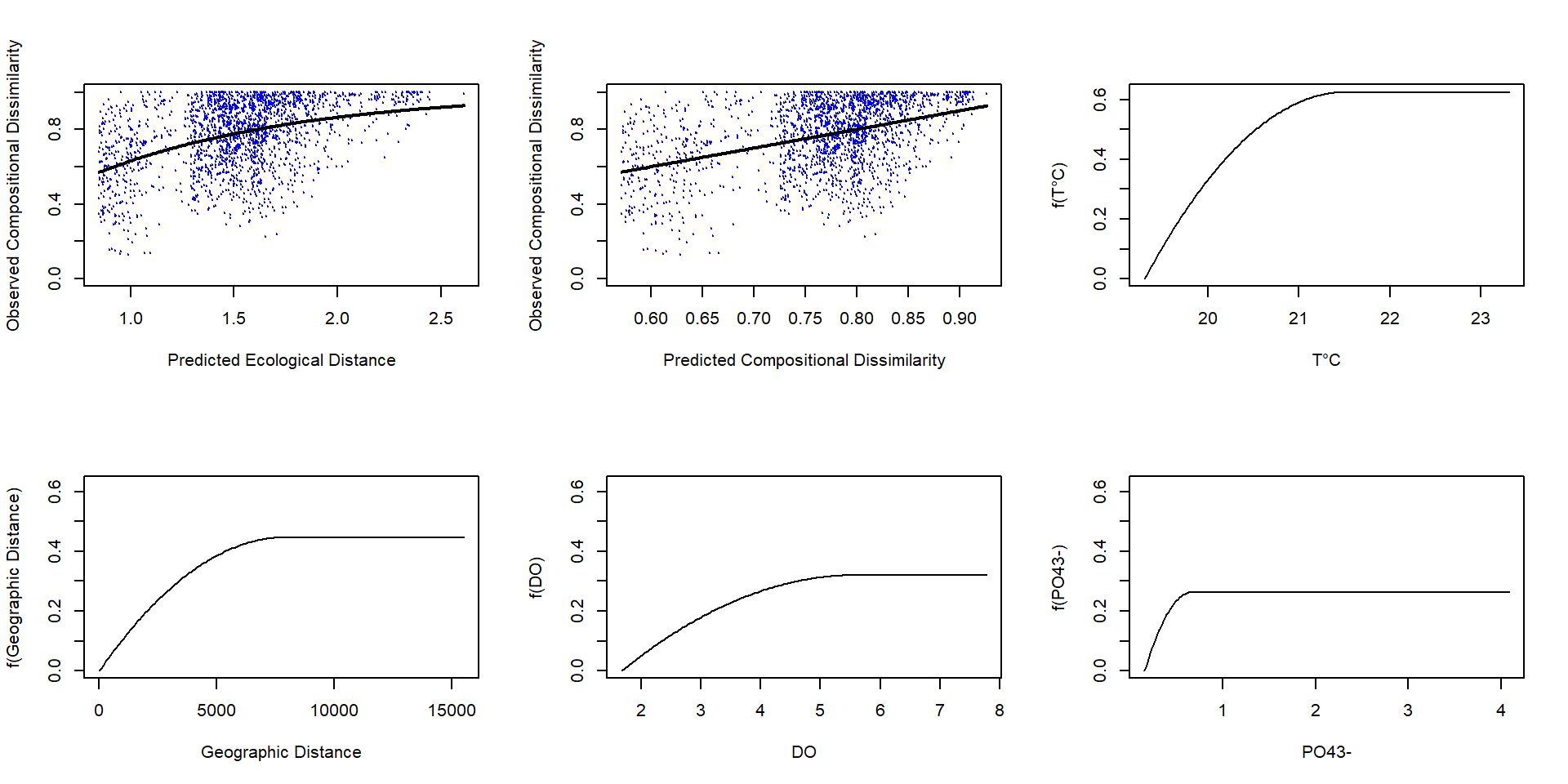
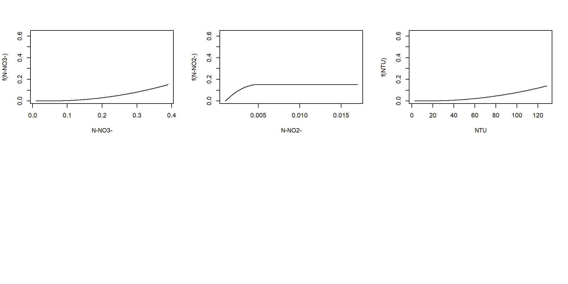
Podemos graficar los resultados del modelo y las curvas i-spline

plot(gdmTab.fit, plot.layout=c(2,3))

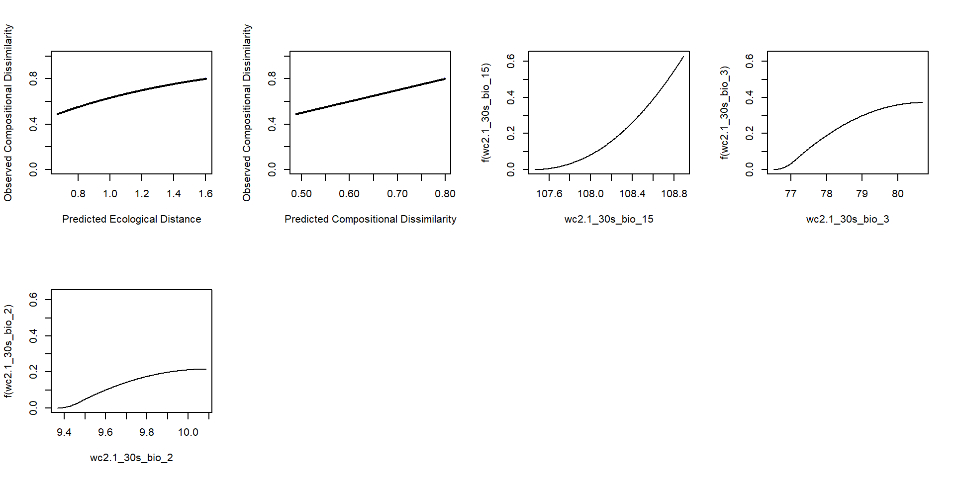
… también las del modelo bioclimático

plot(gdmRast.fit, plot.layout = c(2, 4))

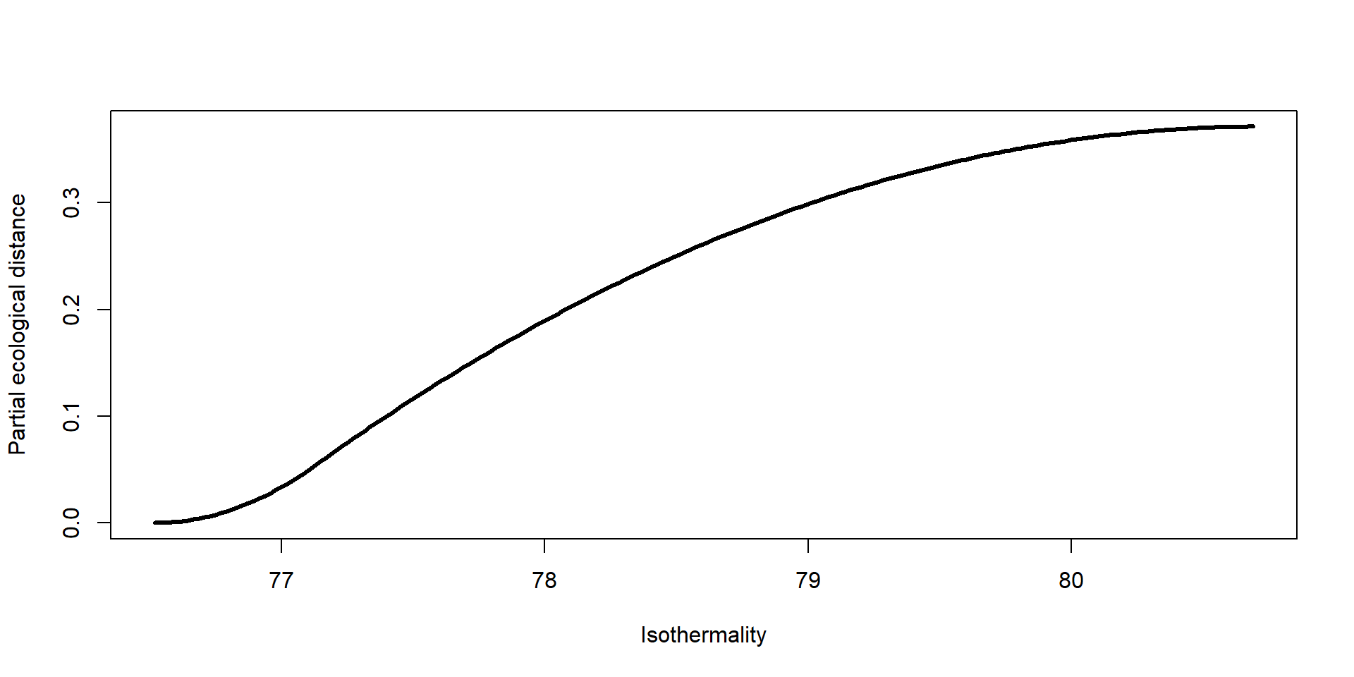
Si necesitamos realizar gráficos independientes, podemos extraer los valores de las curvas i-splines

gdmRast.splines <- isplineExtract(gdmRast.fit)
str(gdmRast.splines)

List of 2
 $ x: num [1:200, 1:20] 3877 3933 3990 4047 4104 ...
  ..- attr(*, "dimnames")=List of 2
  .. ..$ : NULL
  .. ..$ : chr [1:20] "Geographic" "wc2.1_30s_bio_1" "wc2.1_30s_bio_2" "wc2.1_30s_bio_3" ...
 $ y: num [1:200, 1:20] 0 0 0 0 0 0 0 0 0 0 ...
  ..- attr(*, "dimnames")=List of 2
  .. ..$ : NULL
  .. ..$ : chr [1:20] "Geographic" "wc2.1_30s_bio_1" "wc2.1_30s_bio_2" "wc2.1_30s_bio_3" ...

… y posteriormente graficarlas a mano

plot(gdmRast.splines[["x"]][,"wc2.1_30s_bio_3"], 
     gdmRast.splines[["y"]][,"wc2.1_30s_bio_3"], 
     lwd=3,
     type="l", 
     xlab="Isothermality", 
     ylab="Partial ecological distance")

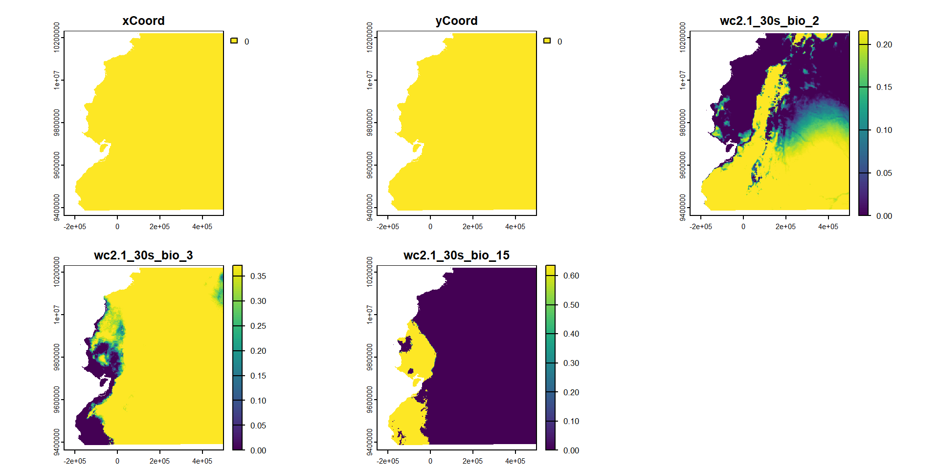
Usemos el modelo para realizar proyecciones

Podemos proyectar el modelo para transformar cada variable ambiental acorde a las i-splines

gdmRast.sp_trans <- gdm.transform(gdmRast.fit, bio)

|---------|---------|---------|---------|
=========================================
                                          

gdmRast.sp_trans

class       : SpatRaster 
size        : 925, 797, 5  (nrow, ncol, nlyr)
resolution  : 940.2445, 940.2445  (x, y)
extent      : -249628.5, 499746.5, 9362131, 10231857  (xmin, xmax, ymin, ymax)
coord. ref. : WGS 84 / UTM zone 18S (EPSG:32718) 
source      : spat_6df41d0fd02_28148_zxzxx9jyyx6UnnI.tif 
names       : xCoord, yCoord, wc2.1_~_bio_2, wc2.1_~_bio_3, wc2.1_~bio_15 
min values  :      0,      0,     0.0000000,     0.0000000,     0.0000000 
max values  :      0,      0,     0.2157599,     0.3712488,     0.6358249 

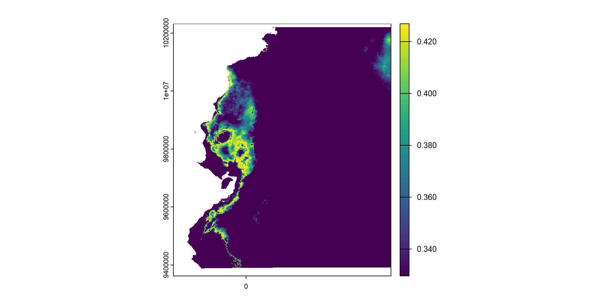
… y graficarlo en forma de mapa

terra::plot(gdmRast.sp_trans)

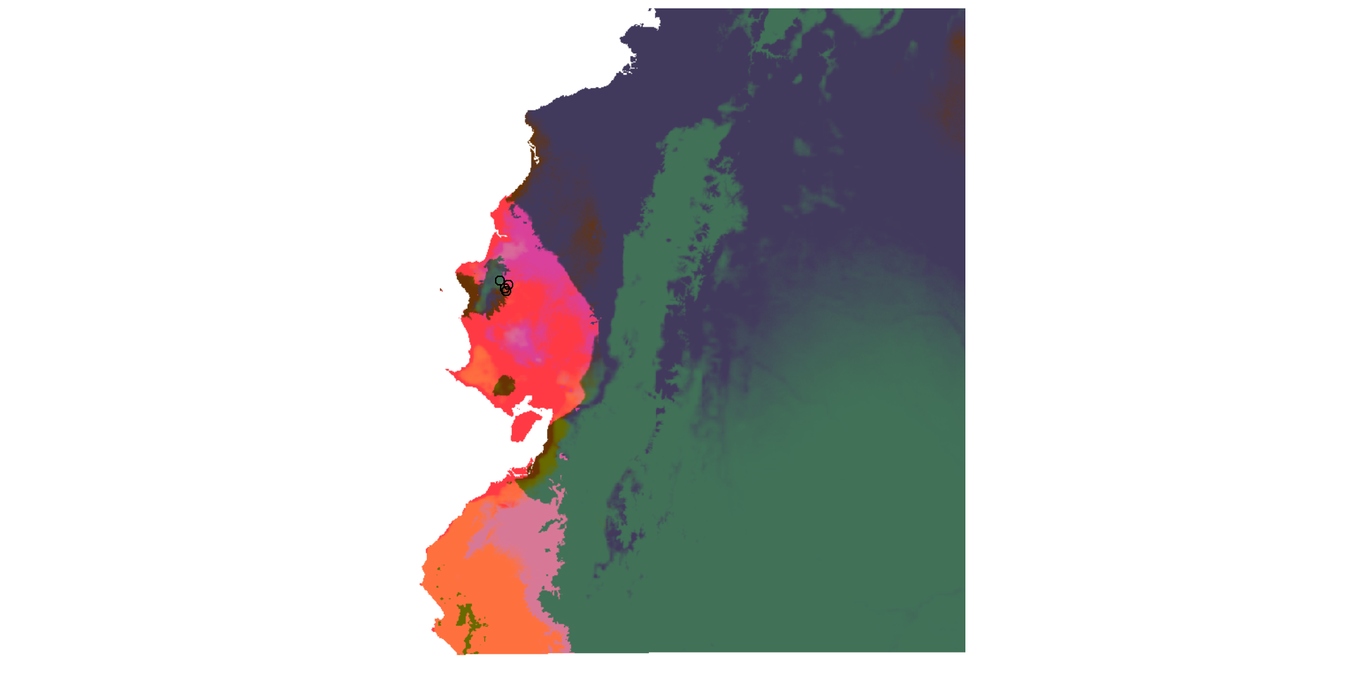
Para reducir la dimensionalidad de las distintas capas, usamos un ACP para seleccionar los tres primeros ejes

pca.rast <- prcomp(gdmRast.sp_trans)

# note the use of the 'index' argument
pca.rast <- terra::predict(gdmRast.sp_trans, pca.rast, index=1:3)

# scale rasters
mnmx <- range(values(pca.rast), na.rm = TRUE)
pca.rast <- ((pca.rast - mnmx[1]) / diff(mnmx)) * 255

pca.rast

class       : SpatRaster 
size        : 925, 797, 3  (nrow, ncol, nlyr)
resolution  : 940.2445, 940.2445  (x, y)
extent      : -249628.5, 499746.5, 9362131, 10231857  (xmin, xmax, ymin, ymax)
coord. ref. : WGS 84 / UTM zone 18S (EPSG:32718) 
source(s)   : memory
names       :       PC1,       PC2,     PC3 
min values  :  65.82556,  51.35117,   0.000 
max values  : 255.00000, 120.79050, 156.447 

Y luego representar cada eje como un componente de color (rojo, azul y verde)

terra::plotRGB(pca.rast, r=1, g=2, b=3)
points(utm[,c("x", "y")])

También podemos analizar cambios en cada pixel entre dos periodos concretos

Primero habrá que generar un objeto raster con los datos climáticos modificados

fut_bioclim <- bio
fut_bioclim[[3]] <- fut_bioclim[[3]] + 1

Posteriormente hacemos la predicción y se dibuja el mapa

timePred <- predict(gdmRast.fit, 
                    bio, 
                    time = T, 
                    predRasts = fut_bioclim)
terra::plot(timePred)