Modelos Generalizados de Disimilitud en R
Generalized Dissimilarity Models (GDM)
Universidad de Córdoba (España)
2024-10-17
Preparando los datos
Usaremos el paquete gdm. Éste tiene una forma particular de funcionar y especificar los datos. Así que necesitamos prepararlos un poco antes de empezar
Cargamos los datos de Michelle, incluyendo las coordenadas geográficas
library(openxlsx)
env <- read.xlsx("data/sciberras_ambiente.xlsx",
                 1,
                 rowNames = TRUE)
com <- read.xlsx("data/sciberras_especies.xlsx",
                 1,
                 rowNames = TRUE)
coords <- read.xlsx("data/sciberras_coords.xlsx",
                    1,
                    rowNames = TRUE)
head(coords)
x y
chapad -57.70311 -38.20977
sauce -61.11647 -38.99773
quequens -60.51297 -38.92499
claromeco -60.08128 -38.86156
quequeng -58.70162 -38.58077
moro -58.40547 -38.50085Cargamos los datos bioclimáticos
En particular cargamos los datos de argentina en formato ráster y en UTM 21s y los recorto para la región de interés
Note
Estos datos los generamos durante la clase sobre análisis de datos espaciales en R.
Reproyecto los datos de coordenadas a UTM 21s y los combino con los datos de comunidades
Important
El paquete gdm requiere que las coordenadas estén especificadas como columnas en la matriz de comunidades, en la matriz de variables ambientales, o en las dos; pero no se pueden especificar como un objeto independiente.
utm <- project(as.matrix(coords),
               from = "EPSG: 4326",
               to = "EPSG:32721")
utm <- data.frame(x = utm[,1],
                  y = utm[,2],
                  rio = rownames(coords))
com$rio <- env$rio
com <- merge(com, utm)
head(com)
rio emertonia sextonis_1 sextonis_2 sextonis_delamarei
1 chapad 0 0 0 0
2 chapad 6 12 0 1
3 chapad 1 4 0 0
4 chapad 0 0 0 0
5 chapad 0 0 0 0
6 chapad 2 0 0 0
halectinosoma_parejae nannopus ectinosomatidae euterpina
1 1 0 0 0
2 1 0 0 0
3 0 0 0 0
4 0 3 0 0
5 0 1 0 0
6 0 10 0 0
quinquelaophonte_aestuarii cyclopoida x y
1 0 0 438444.6 5770677
2 0 0 438444.6 5770677
3 0 0 438444.6 5770677
4 0 0 438444.6 5770677
5 0 0 438444.6 5770677
6 0 0 438444.6 5770677Genero un identificador de sitio común para la matriz de comunidades y la de variables ambientales
              rio sitio     mes materia_org temperatura salinidad   ph site_id
chapad_f_d chapad   des febrero   0.6026517        22.1      1.18 8.71       1
chapad_f_n chapad norte febrero   0.8458035        21.7      2.89 8.61       2
chapad_f_s chapad   sur febrero   0.6467259        22.8      2.86 8.62       3
chapad_j_d chapad   des   julio   0.7584830        11.0      2.20 9.09       4
chapad_j_n chapad norte   julio   0.8047438        10.8      3.20 9.07       5
chapad_j_s chapad   sur   julio   0.7331378        12.4      0.98 9.07       6
Calibrando modelos GDM
Usamos el paquete gdm
Creamos la tabla de disimilaridades
library(gdm)
gdmTab <- formatsitepair(com[,-1], # Quito la columna `río`
               bioFormat = 1,
               abundance = TRUE,
               XColumn = "x", # Nombre de la coordenada X
               YColumn = "y", # Nombre de la coordenada Y
               siteColumn = "site_id", # Nombre del identificador
               predData = env[,-c(1:3)]) # Quito columnas de texto

gdmRast <- formatsitepair(com[,-1],
               bioFormat = 1,
               abundance = TRUE,
               XColumn = "x",
               YColumn = "y",
               siteColumn = "site_id",
               predData = bioclim)

head(gdmTab)
distance weights s1.xCoord s1.yCoord s2.xCoord s2.yCoord
chapad_f_d 0.9047619 1 438444.6 5770677 438444.6 5770677
chapad_f_d.1 1.0000000 1 438444.6 5770677 438444.6 5770677
chapad_f_d.2 1.0000000 1 438444.6 5770677 438444.6 5770677
chapad_f_d.3 1.0000000 1 438444.6 5770677 438444.6 5770677
chapad_f_d.4 1.0000000 1 438444.6 5770677 438444.6 5770677
chapad_f_d.5 1.0000000 1 438444.6 5770677 438444.6 5770677
s1.materia_org s1.temperatura s1.salinidad s1.ph s2.materia_org
chapad_f_d 0.6026517 22.1 1.18 8.71 0.8458035
chapad_f_d.1 0.6026517 22.1 1.18 8.71 0.6467259
chapad_f_d.2 0.6026517 22.1 1.18 8.71 0.7584830
chapad_f_d.3 0.6026517 22.1 1.18 8.71 0.8047438
chapad_f_d.4 0.6026517 22.1 1.18 8.71 0.7331378
chapad_f_d.5 0.6026517 22.1 1.18 8.71 0.8279125
s2.temperatura s2.salinidad s2.ph
chapad_f_d 21.7 2.89 8.61
chapad_f_d.1 22.8 2.86 8.62
chapad_f_d.2 11.0 2.20 9.09
chapad_f_d.3 10.8 3.20 9.07
chapad_f_d.4 12.4 0.98 9.07
chapad_f_d.5 17.2 2.49 8.90Calibramos los modelos
Analicemos los resultados
Veamos los resultados de los datos de Michelle
[1]
[1]
[1] GDM Modelling Summary
[1] Creation Date:  Thu Oct 24 23:43:17 2024
[1]
[1] Name:  gdmTab.fit
[1]
[1] Data:  gdmTab
[1]
[1] Samples:  2485
[1]
[1] Geographical distance used in model fitting?  TRUE
[1]
[1] NULL Deviance:  884.14
[1] GDM Deviance:  851.866
[1] Percent Deviance Explained:  3.65
[1]
[1] Intercept:  1.437
[1]
[1] PREDICTOR ORDER BY SUM OF I-SPLINE COEFFICIENTS:
[1]
[1] Predictor 1: ph
[1] Splines: 3
[1] Min Knot: 7.27
[1] 50% Knot: 8.85
[1] Max Knot: 9.66
[1] Coefficient[1]: 0
[1] Coefficient[2]: 0
[1] Coefficient[3]: 0.98
[1] Sum of coefficients for ph: 0.98
[1]
[1] Predictor 2: materia_org
[1] Splines: 3
[1] Min Knot: 0.34
[1] 50% Knot: 0.675
[1] Max Knot: 1.37
[1] Coefficient[1]: 0
[1] Coefficient[2]: 0.391
[1] Coefficient[3]: 0.326
[1] Sum of coefficients for materia_org: 0.718
[1]
[1] Predictor 3: salinidad
[1] Splines: 3
[1] Min Knot: 0.15
[1] 50% Knot: 2.67
[1] Max Knot: 3.49
[1] Coefficient[1]: 0.436
[1] Coefficient[2]: 0
[1] Coefficient[3]: 0
[1] Sum of coefficients for salinidad: 0.436
[1]
[1] Predictor 4: Geographic
[1] Splines: 3
[1] Min Knot: 0
[1] 50% Knot: 96436.034
[1] Max Knot: 309976.305
[1] Coefficient[1]: 0
[1] Coefficient[2]: 0.136
[1] Coefficient[3]: 0
[1] Sum of coefficients for Geographic: 0.136
[1]
[1] Predictor 5: temperatura
[1] Splines: 3
[1] Min Knot: 6.5
[1] 50% Knot: 17.2
[1] Max Knot: 24
[1] Coefficient[1]: 0
[1] Coefficient[2]: 0
[1] Coefficient[3]: 0
[1] Sum of coefficients for temperatura: 0
… y los del modelo calibrado con variables bioclimáticas
[1]
[1]
[1] GDM Modelling Summary
[1] Creation Date:  Thu Oct 24 23:43:17 2024
[1]
[1] Name:  gdmRast.fit
[1]
[1] Data:  gdmRast
[1]
[1] Samples:  28
[1]
[1] Geographical distance used in model fitting?  TRUE
[1]
[1] NULL Deviance:  7.644
[1] GDM Deviance:  1.315
[1] Percent Deviance Explained:  82.803
[1]
[1] Intercept:  0.163
[1]
[1] PREDICTOR ORDER BY SUM OF I-SPLINE COEFFICIENTS:
[1]
[1] Predictor 1: bio1
[1] Splines: 3
[1] Min Knot: 14.108
[1] 50% Knot: 14.234
[1] Max Knot: 14.463
[1] Coefficient[1]: 0.673
[1] Coefficient[2]: 0.931
[1] Coefficient[3]: 0
[1] Sum of coefficients for bio1: 1.603
[1]
[1] Predictor 2: bio10
[1] Splines: 3
[1] Min Knot: 19.769
[1] 50% Knot: 20.108
[1] Max Knot: 20.521
[1] Coefficient[1]: 0.915
[1] Coefficient[2]: 0
[1] Coefficient[3]: 0
[1] Sum of coefficients for bio10: 0.915
[1]
[1] Predictor 3: bio11
[1] Splines: 3
[1] Min Knot: 8.418
[1] 50% Knot: 8.574
[1] Max Knot: 8.888
[1] Coefficient[1]: 0.474
[1] Coefficient[2]: 0
[1] Coefficient[3]: 0
[1] Sum of coefficients for bio11: 0.474
[1]
[1] Predictor 4: bio16
[1] Splines: 3
[1] Min Knot: 234
[1] 50% Knot: 260.931
[1] Max Knot: 264.396
[1] Coefficient[1]: 0
[1] Coefficient[2]: 0
[1] Coefficient[3]: 0.282
[1] Sum of coefficients for bio16: 0.282
[1]
[1] Predictor 5: bio5
[1] Splines: 3
[1] Min Knot: 26.8
[1] 50% Knot: 26.99
[1] Max Knot: 28.2
[1] Coefficient[1]: 0.149
[1] Coefficient[2]: 0
[1] Coefficient[3]: 0
[1] Sum of coefficients for bio5: 0.149
[1]
[1] Predictor 6: Geographic
[1] Splines: 3
[1] Min Knot: 13038.405
[1] 50% Knot: 137784.596
[1] Max Knot: 309919.344
[1] Coefficient[1]: 0
[1] Coefficient[2]: 0
[1] Coefficient[3]: 0
[1] Sum of coefficients for Geographic: 0
[1]
[1] Predictor 7: bio2
[1] Splines: 3
[1] Min Knot: 10.662
[1] 50% Knot: 11.037
[1] Max Knot: 12.348
[1] Coefficient[1]: 0
[1] Coefficient[2]: 0
[1] Coefficient[3]: 0
[1] Sum of coefficients for bio2: 0
[1]
[1] Predictor 8: bio3
[1] Splines: 3
[1] Min Knot: 46.564
[1] 50% Knot: 47.057
[1] Max Knot: 48.5
[1] Coefficient[1]: 0
[1] Coefficient[2]: 0
[1] Coefficient[3]: 0
[1] Sum of coefficients for bio3: 0
[1]
[1] Predictor 9: bio4
[1] Splines: 3
[1] Min Knot: 458.967
[1] 50% Knot: 465.266
[1] Max Knot: 497.734
[1] Coefficient[1]: 0
[1] Coefficient[2]: 0
[1] Coefficient[3]: 0
[1] Sum of coefficients for bio4: 0
[1]
[1] Predictor 10: bio6
[1] Splines: 3
[1] Min Knot: 2.739
[1] 50% Knot: 3.496
[1] Max Knot: 4.183
[1] Coefficient[1]: 0
[1] Coefficient[2]: 0
[1] Coefficient[3]: 0
[1] Sum of coefficients for bio6: 0
[1]
[1] Predictor 11: bio7
[1] Splines: 3
[1] Min Knot: 22.897
[1] 50% Knot: 23.354
[1] Max Knot: 25.461
[1] Coefficient[1]: 0
[1] Coefficient[2]: 0
[1] Coefficient[3]: 0
[1] Sum of coefficients for bio7: 0
[1]
[1] Predictor 12: bio8
[1] Splines: 3
[1] Min Knot: 15.425
[1] 50% Knot: 17.728
[1] Max Knot: 18.157
[1] Coefficient[1]: 0
[1] Coefficient[2]: 0
[1] Coefficient[3]: 0
[1] Sum of coefficients for bio8: 0
[1]
[1] Predictor 13: bio9
[1] Splines: 3
[1] Min Knot: 8.418
[1] 50% Knot: 9.225
[1] Max Knot: 11.148
[1] Coefficient[1]: 0
[1] Coefficient[2]: 0
[1] Coefficient[3]: 0
[1] Sum of coefficients for bio9: 0
[1]
[1] Predictor 14: bio12
[1] Splines: 3
[1] Min Knot: 699.39
[1] 50% Knot: 868.324
[1] Max Knot: 894.967
[1] Coefficient[1]: 0
[1] Coefficient[2]: 0
[1] Coefficient[3]: 0
[1] Sum of coefficients for bio12: 0
[1]
[1] Predictor 15: bio13
[1] Splines: 3
[1] Min Knot: 84
[1] 50% Knot: 91.043
[1] Max Knot: 99
[1] Coefficient[1]: 0
[1] Coefficient[2]: 0
[1] Coefficient[3]: 0
[1] Sum of coefficients for bio13: 0
[1]
[1] Predictor 16: bio14
[1] Splines: 3
[1] Min Knot: 31.893
[1] 50% Knot: 47.5
[1] Max Knot: 51
[1] Coefficient[1]: 0
[1] Coefficient[2]: 0
[1] Coefficient[3]: 0
[1] Sum of coefficients for bio14: 0
[1]
[1] Predictor 17: bio15
[1] Splines: 3
[1] Min Knot: 16.886
[1] 50% Knot: 18.46
[1] Max Knot: 30.844
[1] Coefficient[1]: 0
[1] Coefficient[2]: 0
[1] Coefficient[3]: 0
[1] Sum of coefficients for bio15: 0
[1]
[1] Predictor 18: bio17
[1] Splines: 3
[1] Min Knot: 101.893
[1] 50% Knot: 169.586
[1] Max Knot: 174
[1] Coefficient[1]: 0
[1] Coefficient[2]: 0
[1] Coefficient[3]: 0
[1] Sum of coefficients for bio17: 0
[1]
[1] Predictor 19: bio18
[1] Splines: 3
[1] Min Knot: 208.392
[1] 50% Knot: 234.903
[1] Max Knot: 245.588
[1] Coefficient[1]: 0
[1] Coefficient[2]: 0
[1] Coefficient[3]: 0
[1] Sum of coefficients for bio18: 0
[1]
[1] Predictor 20: bio19
[1] Splines: 3
[1] Min Knot: 101.893
[1] 50% Knot: 176.446
[1] Max Knot: 204.367
[1] Coefficient[1]: 0
[1] Coefficient[2]: 0
[1] Coefficient[3]: 0
[1] Sum of coefficients for bio19: 0
Important
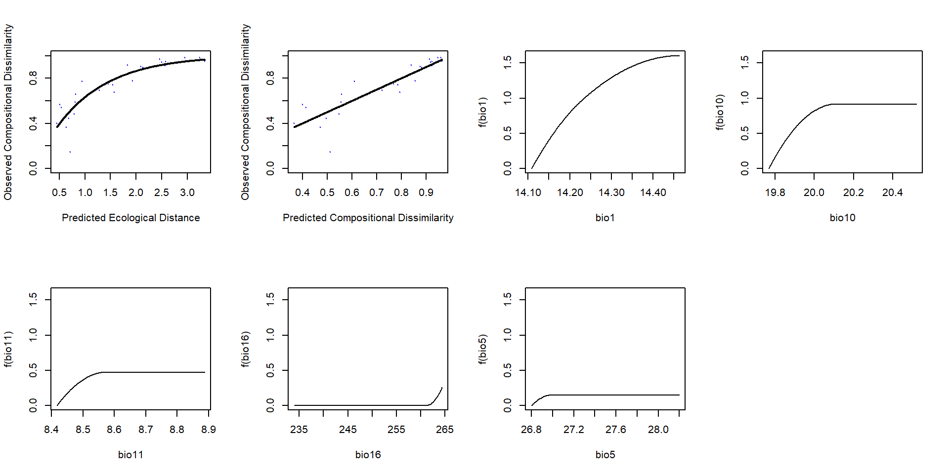
Fijaros como el modelo explica un 80% de la desvianza de los datos. Pero tiene un poco de truco, ya que este modelo solo contempla el río como unidad de muestreo, al caer las 3 parcelas (desembocadura, norte y sur) en el mismo pixel.
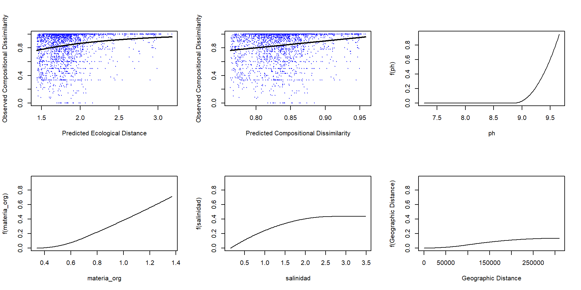
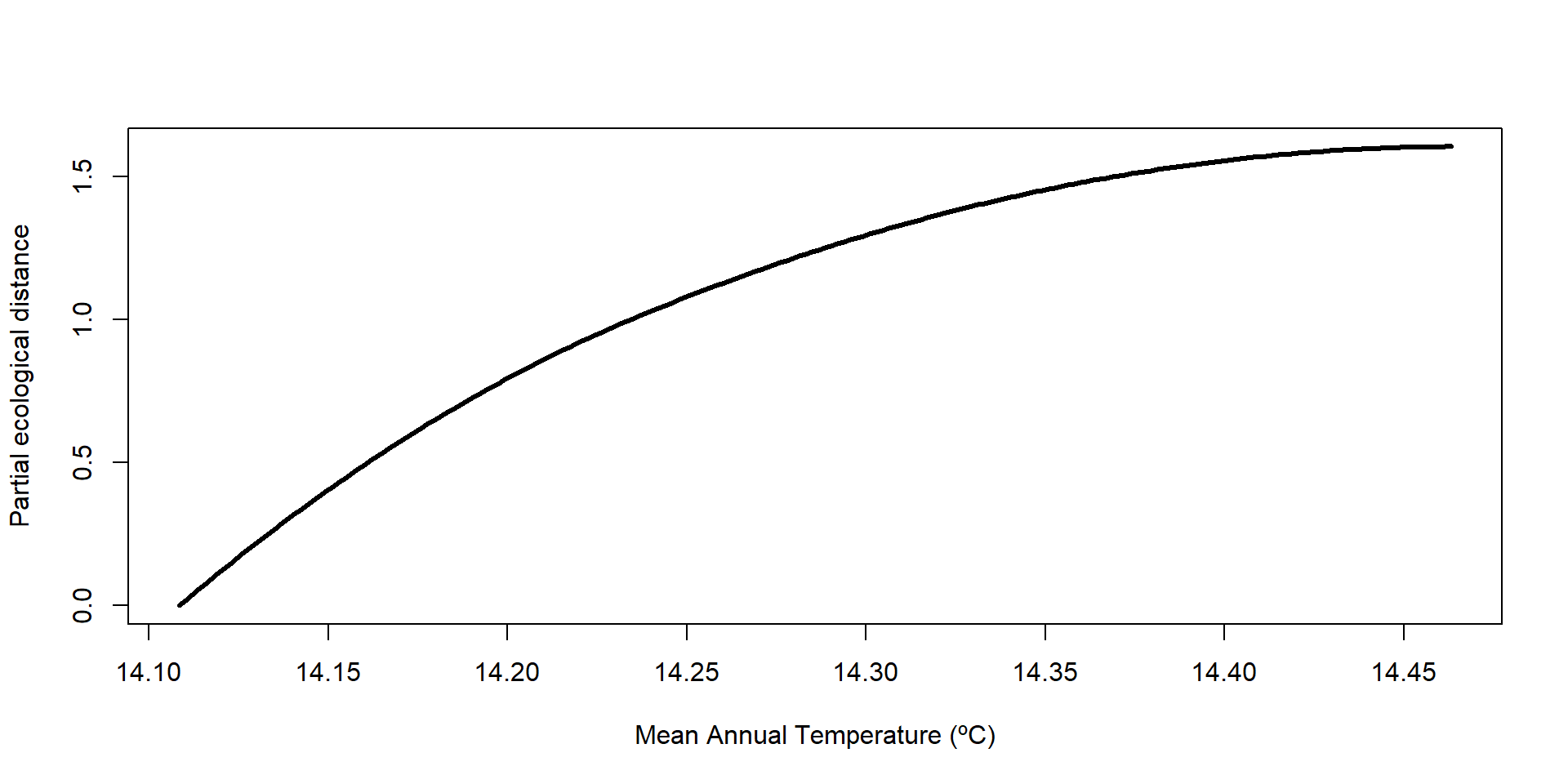
Podemos graficar los resultados del modelo y las curvas i-spline
… también las del modelo bioclimático
Si necesitamos realizar gráficos independientes, podemos extraer los valores de las curvas i-splines
List of 2
 $ x: num [1:200, 1:20] 13038 14530 16022 17514 19006 ...
  ..- attr(*, "dimnames")=List of 2
  .. ..$ : NULL
  .. ..$ : chr [1:20] "Geographic" "bio1" "bio2" "bio3" ...
 $ y: num [1:200, 1:20] 0 0 0 0 0 0 0 0 0 0 ...
  ..- attr(*, "dimnames")=List of 2
  .. ..$ : NULL
  .. ..$ : chr [1:20] "Geographic" "bio1" "bio2" "bio3" ...
… y posteriormente graficarlas a mano
Usemos el modelo para realizar proyecciones
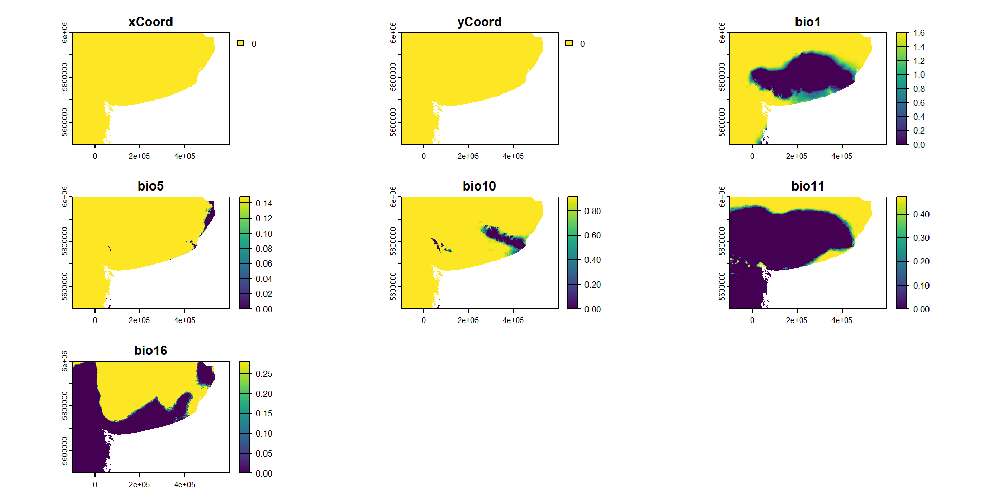
Podemos proyectar el modelo para transformar cada variable ambiental acorde a las i-splines
|---------|---------|---------|---------|
=========================================
class : SpatRaster
dimensions : 500, 700, 7 (nrow, ncol, nlyr)
resolution : 1000, 1000 (x, y)
extent : -100055.4, 599944.6, 5500177, 6000177 (xmin, xmax, ymin, ymax)
coord. ref. : WGS 84 / UTM zone 21S (EPSG:32721)
source : spat_183429d35181_6196_o8up7yuDdJ6XHBX.tif
names : xCoord, yCoord, bio1, bio5, bio10, bio11, ...
min values : 0, 0, 0.000000, 0.0000000, 0.0000000, 0.0000000, ...
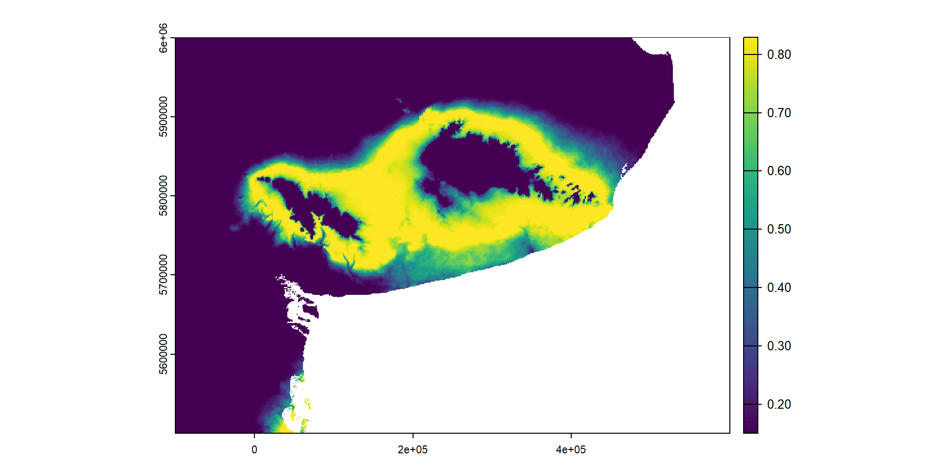
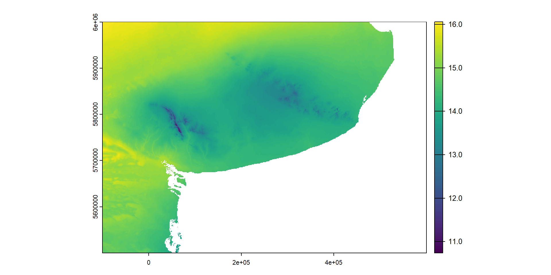
max values : 0, 0, 1.603295, 0.1485767, 0.9152355, 0.4735476, ... … y graficarlo en forma de mapa
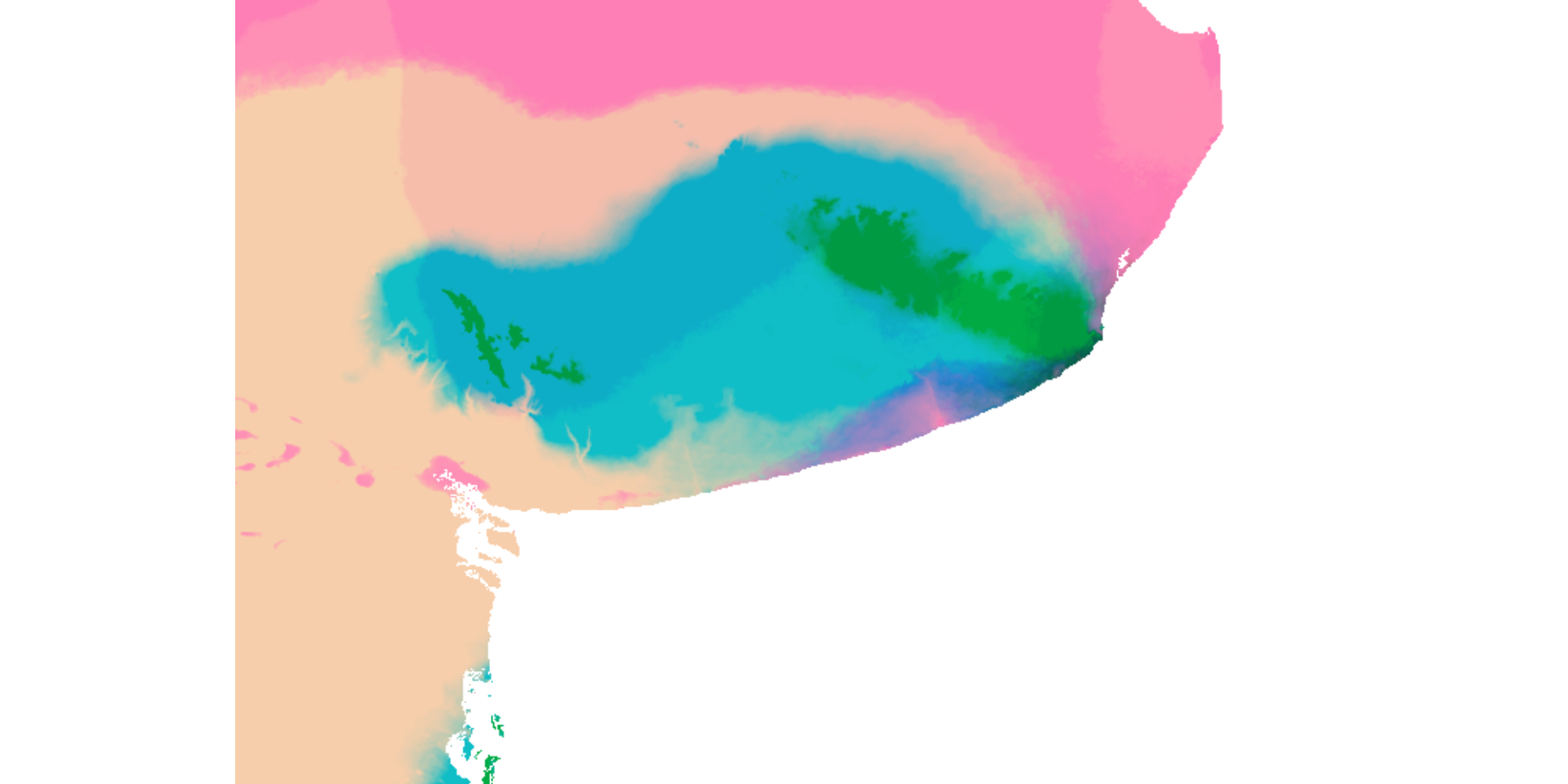
Para reducir la dimensionalidad de las distintas capas, usamos un ACP para seleccionar los tres primeros ejes
pca.rast <- prcomp(gdmRast.sp_trans)

# note the use of the 'index' argument
pca.rast <- terra::predict(gdmRast.sp_trans, pca.rast, index=1:3)

# scale rasters
mnmx <- range(values(pca.rast), na.rm = TRUE)
pca.rast <- ((pca.rast - mnmx[1]) / diff(mnmx)) * 255

pca.rast
class : SpatRaster
dimensions : 500, 700, 3 (nrow, ncol, nlyr)
resolution : 1000, 1000 (x, y)
extent : -100055.4, 599944.6, 5500177, 6000177 (xmin, xmax, ymin, ymax)
coord. ref. : WGS 84 / UTM zone 21S (EPSG:32721)
source(s) : memory
names : PC1, PC2, PC3
min values : 0, 91.78841, 67.39197
max values : 255, 206.29877, 207.57428 Y luego representar cada eje como un componente de color (rojo, azul y verde)
También podemos analizar cambios en cada pixel entre dos periodos concretos
Primero habrá que generar un objeto raster con los datos climáticos modificados