Modelos Jerárquicos de Comunidades de Especies en R
Hierarchical Models of Species Communities (HMSC)
2024-10-18
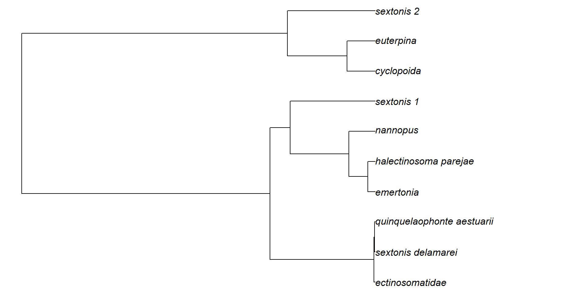
Simulamos unos datos filogenéticos
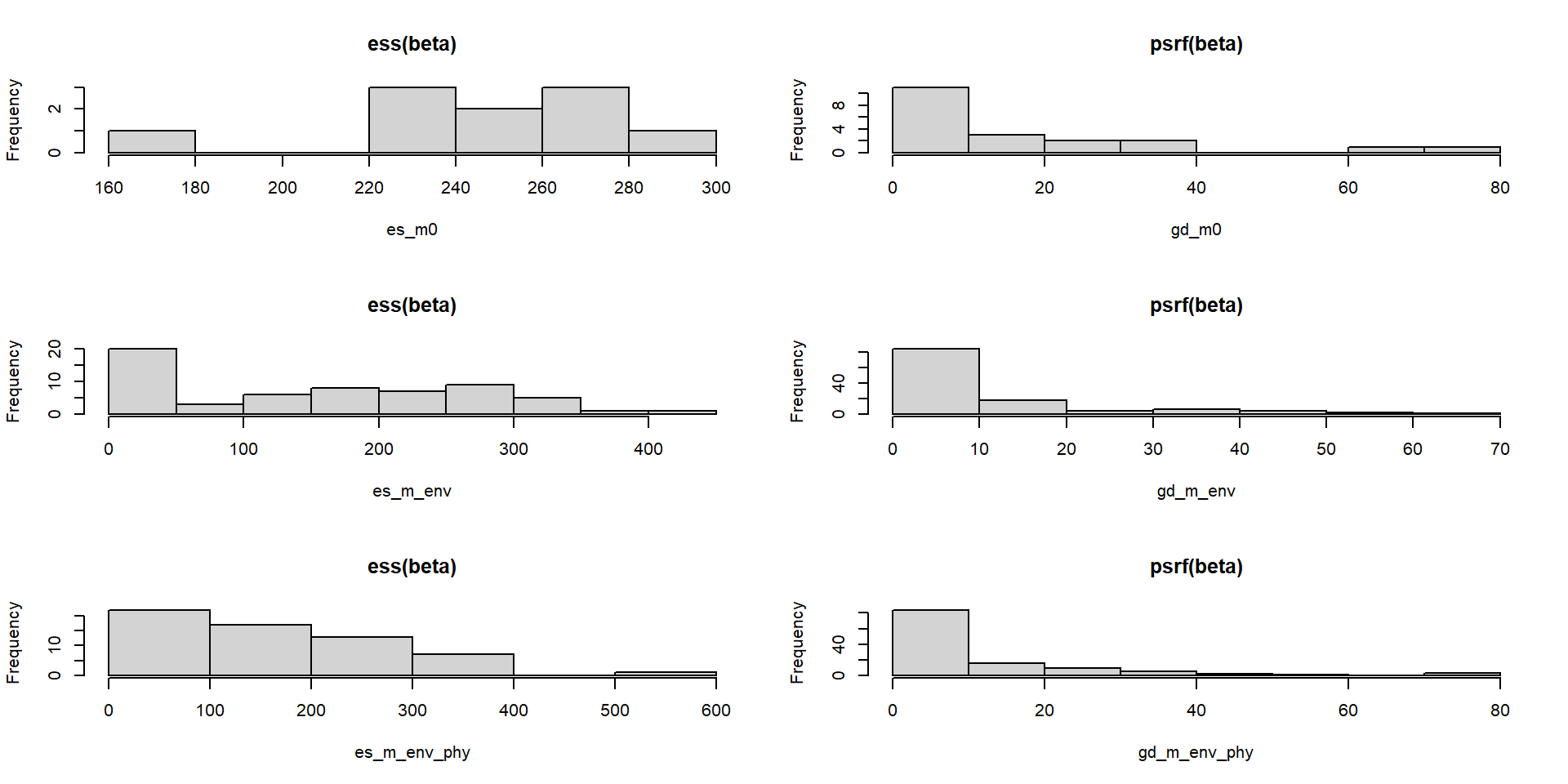
Dibujamos las gráficas de esos dos parámetros
Effective size debería estar entorno al número de muestras de las MCMC (samples * nChains). El diagnóstico de Gelman debería estar entorno a 1.
… lo mismo pero con los valores de Omega, que son los coeficientes de interacciones entre especies
par(mfrow=c(3,2))
hist(effectiveSize(mpost_m0$Omega[[1]]), main="ess(omega)")
hist(gelman.diag(mpost_m0$Omega[[1]], multivariate=FALSE)$psrf, main="psrf(omega)")
hist(effectiveSize(mpost_m_env$Omega[[1]]), main="ess(omega)")
hist(gelman.diag(mpost_m_env$Omega[[1]], multivariate=FALSE)$psrf, main="psrf(omega)")
hist(effectiveSize(mpost_m_env_phy$Omega[[1]]), main="ess(omega)")
hist(gelman.diag(mpost_m_env_phy$Omega[[1]], multivariate=FALSE)$psrf, main="psrf(omega)")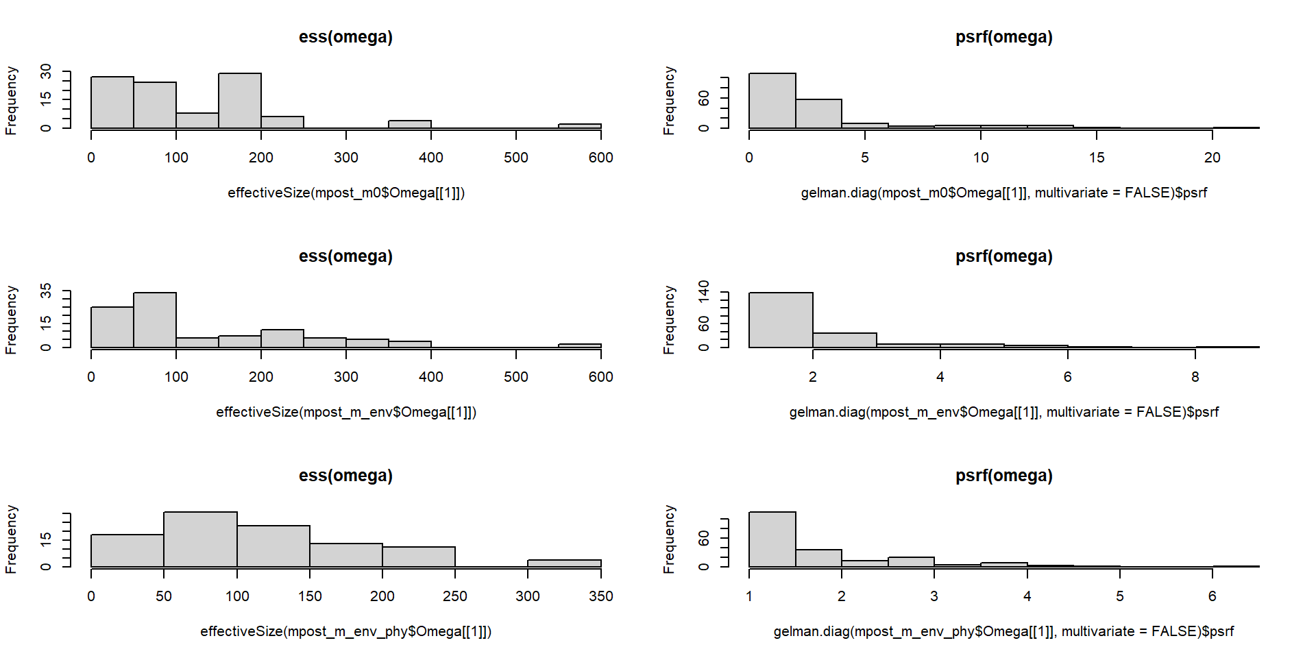
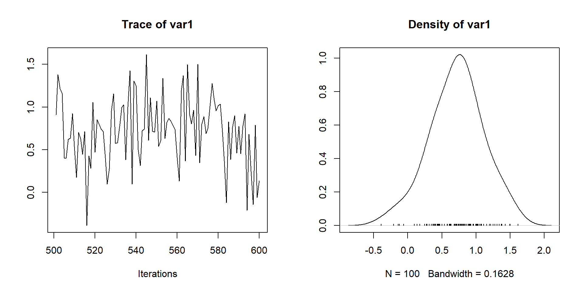
Tambien podemos dibujar algunas de las cadenas para visulizar su forma y ver si se han estabilizado
Una vez que tengamos un modelo sólido. Nos interesa ver que papel juegan las variables ambientales en las especies/comunidades.
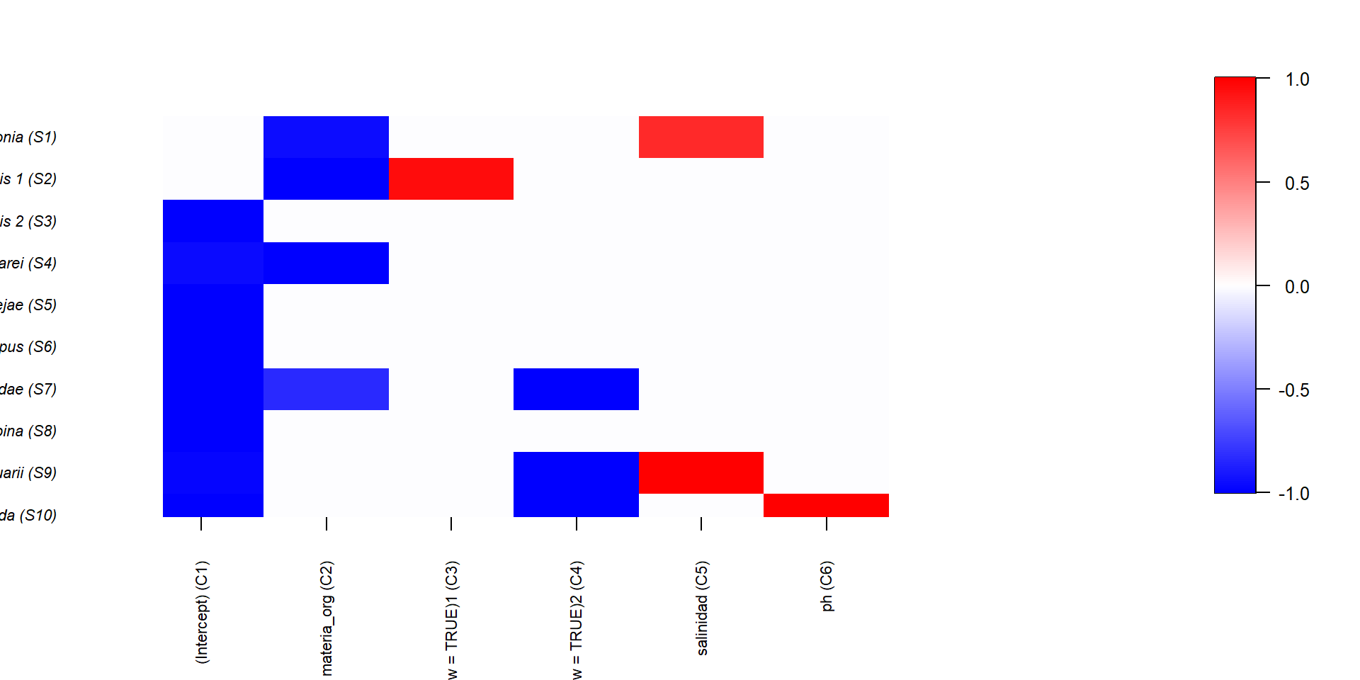
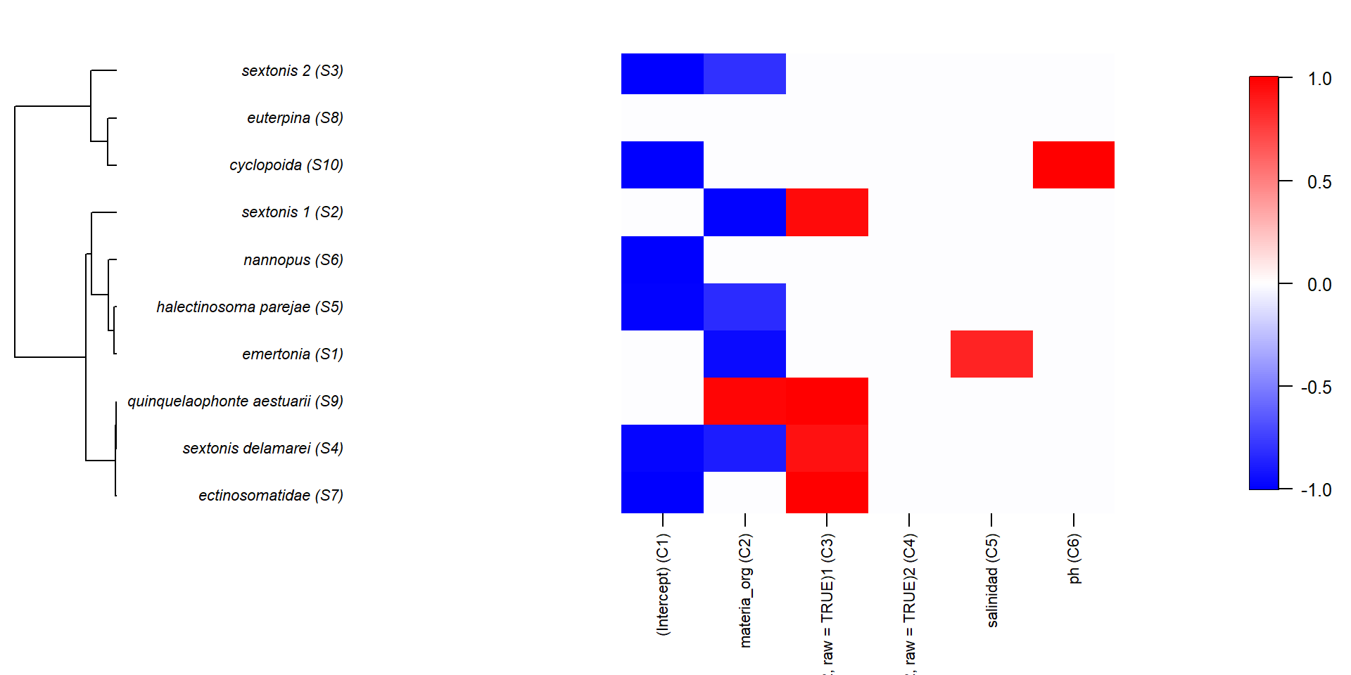
También podemos ver su relación con la información filogenética, si la hemos incluido en el modelo
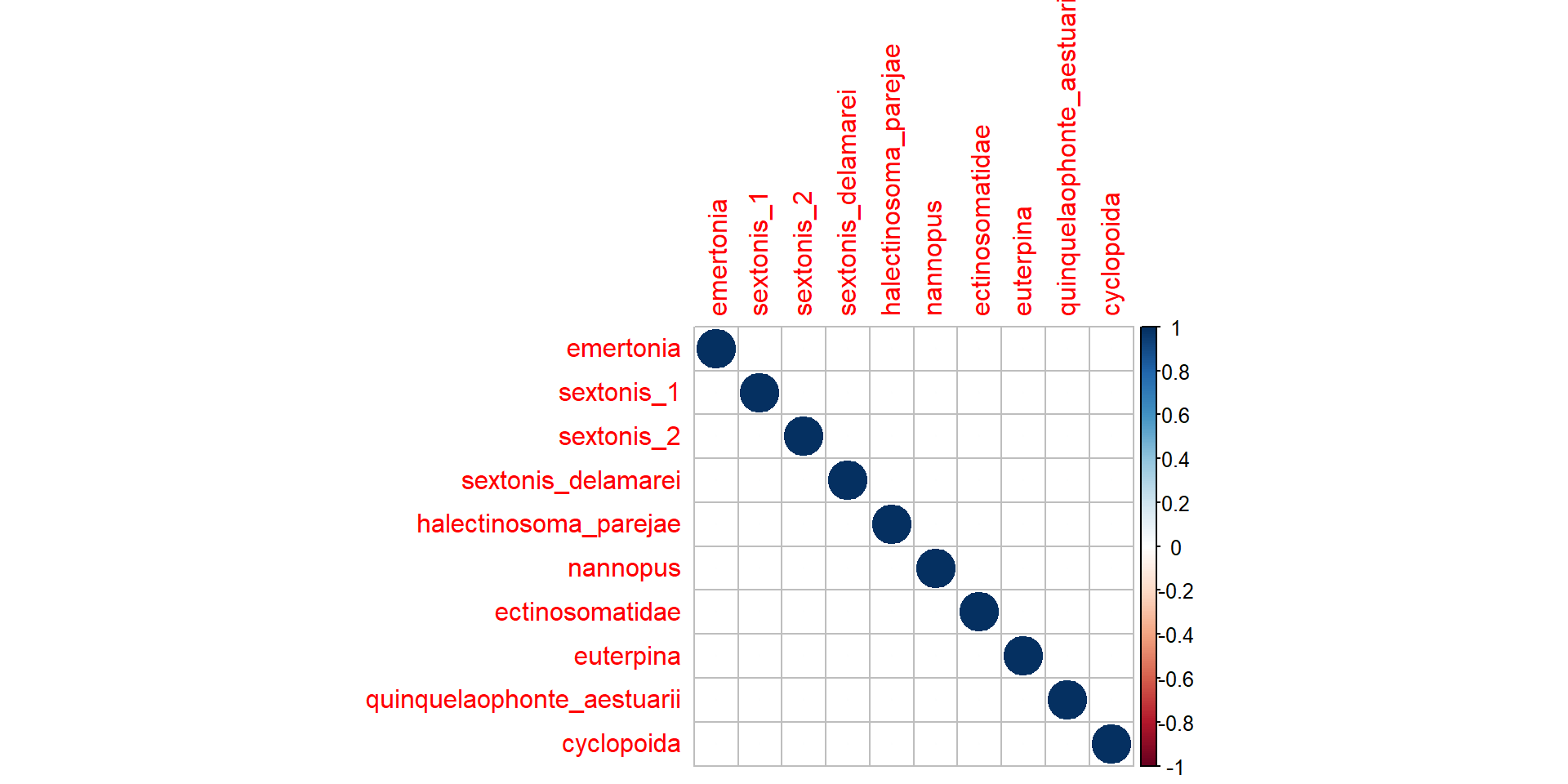
Otro aspecto importante/novedoso es estimar las correlaciones entre especies
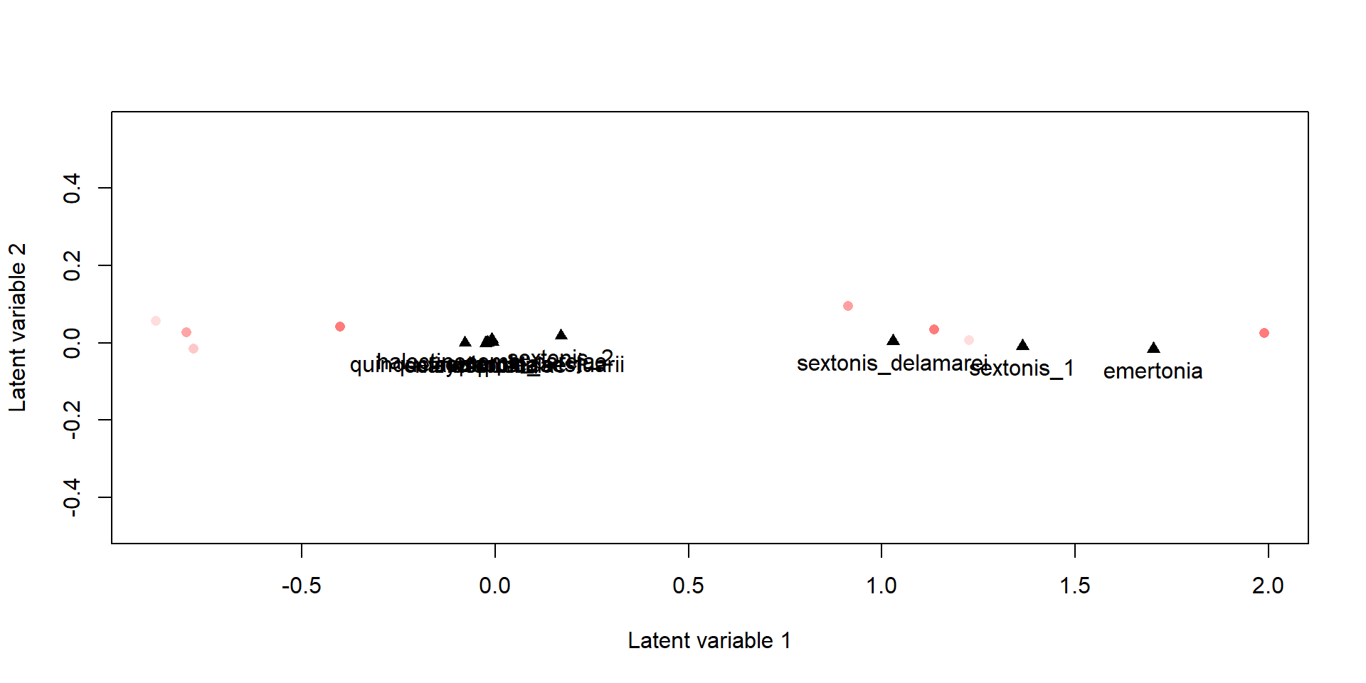
Cuando especificamos un modelo sin variables ambientales, estamos haciendo un modelo “unconstrained” o indirecto. Por lo que se puede usar para generar gráficos de ordenación.
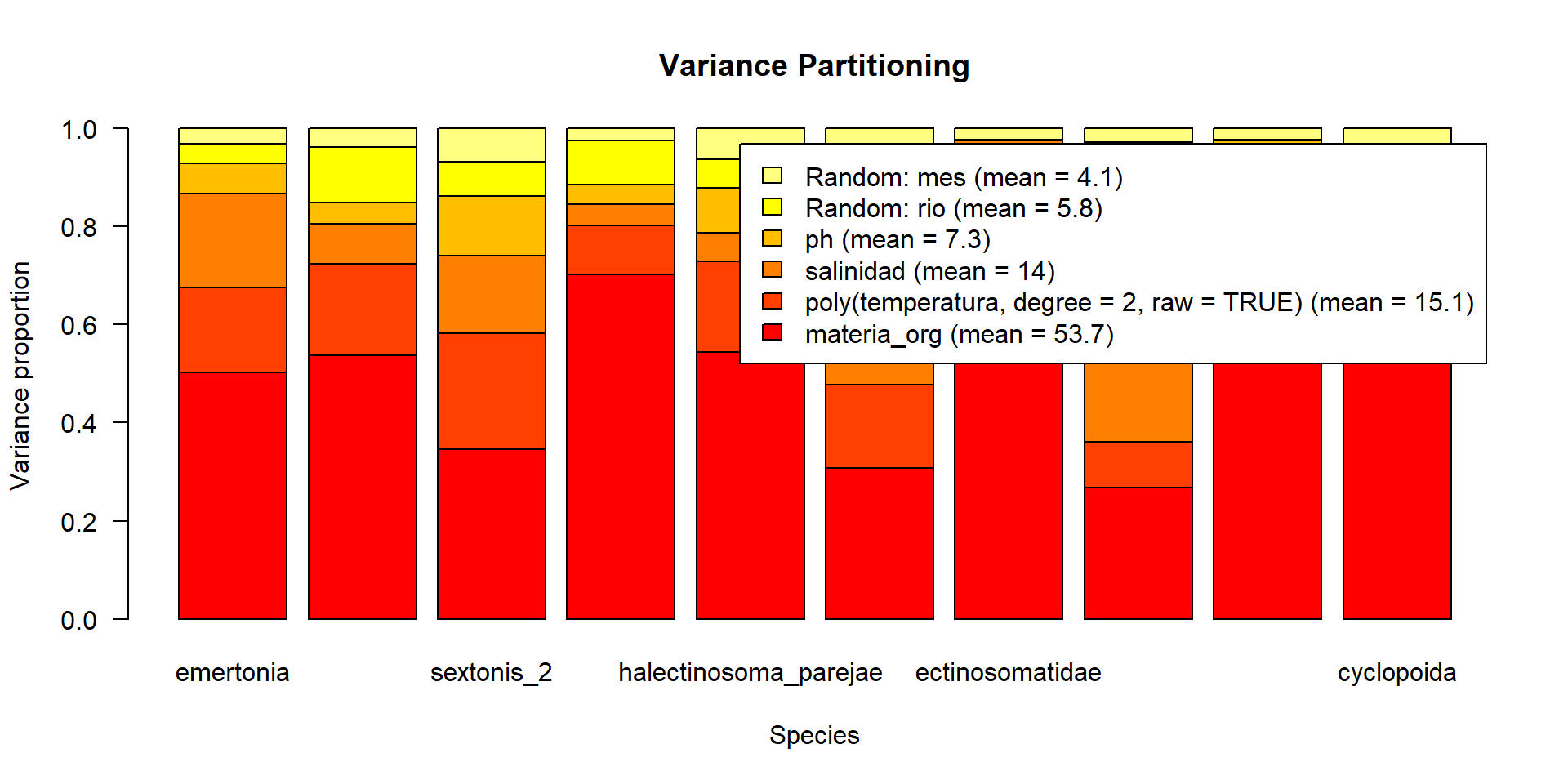
En este tipo de modelos, la importancia de cada variable se mide en términos de variación explicada y se calcula con análisis de particionado de la varianza
Como en los Modelos de Distribución de Especies, podemos calcular curvas de respuesta de cada especie/comunidad a las variables ambientales
Gradient = constructGradient(m1, focalVariable = "temperatura",
non.focalVariables = list("habitat"=list(3,"open")))
Gradient$XDataNew
temperatura materia_org salinidad ph
1 -2.065315281 -0.1667234554 -0.501380262 0.37285247
2 -1.878146837 -0.1516142030 -0.455942859 0.33906285
3 -1.690978393 -0.1365049507 -0.410505456 0.30527323
4 -1.503809949 -0.1213956984 -0.365068052 0.27148361
5 -1.316641505 -0.1062864460 -0.319630649 0.23769400
6 -1.129473060 -0.0911771937 -0.274193245 0.20390438
7 -0.942304616 -0.0760679413 -0.228755842 0.17011476
8 -0.755136172 -0.0609586890 -0.183318438 0.13632514
9 -0.567967728 -0.0458494366 -0.137881035 0.10253552
10 -0.380799284 -0.0307401843 -0.092443632 0.06874590
11 -0.193630840 -0.0156309320 -0.047006228 0.03495628
12 -0.006462395 -0.0005216796 -0.001568825 0.00116666
13 0.180706049 0.0145875727 0.043868579 -0.03262296
14 0.367874493 0.0296968251 0.089305982 -0.06641258
15 0.555042937 0.0448060774 0.134743386 -0.10020220
16 0.742211381 0.0599153298 0.180180789 -0.13399182
17 0.929379825 0.0750245821 0.225618193 -0.16778144
18 1.116548270 0.0901338344 0.271055596 -0.20157106
19 1.303716714 0.1052430868 0.316492999 -0.23536068
20 1.490885158 0.1203523391 0.361930403 -0.26915030predY <- predict(m1,
XData=Gradient$XDataNew,
studyDesign=Gradient$studyDesignNew,
ranLevels=Gradient$rLNew,
expected=TRUE)
plotGradient(m1, Gradient, pred=predY, measure="S")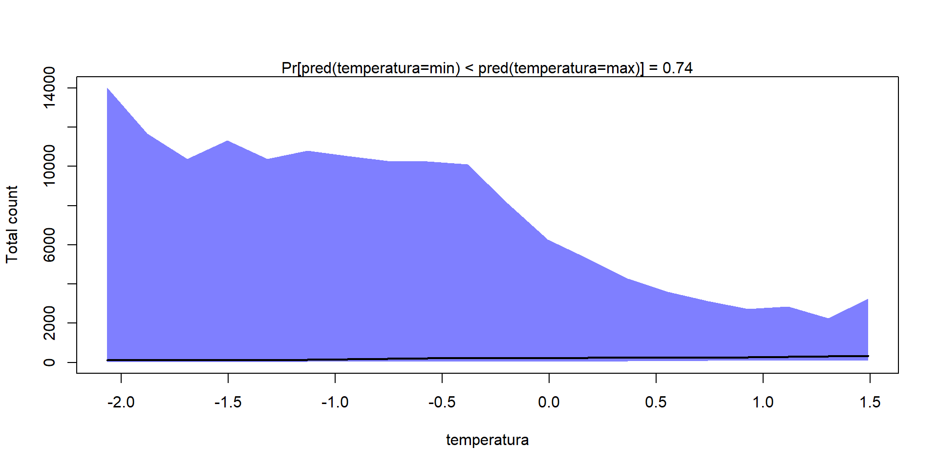
[1] 0.74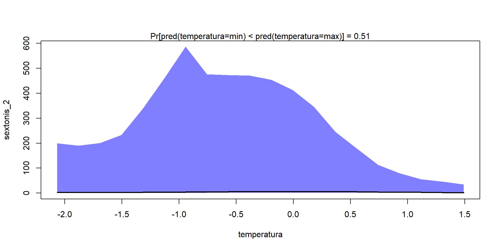
[1] 0.5125