2. Combine dsclim data from past to future
Source:vignettes/a2_dsclim_past_to_future.Rmd
a2_dsclim_past_to_future.RmdLoading past data into R environment
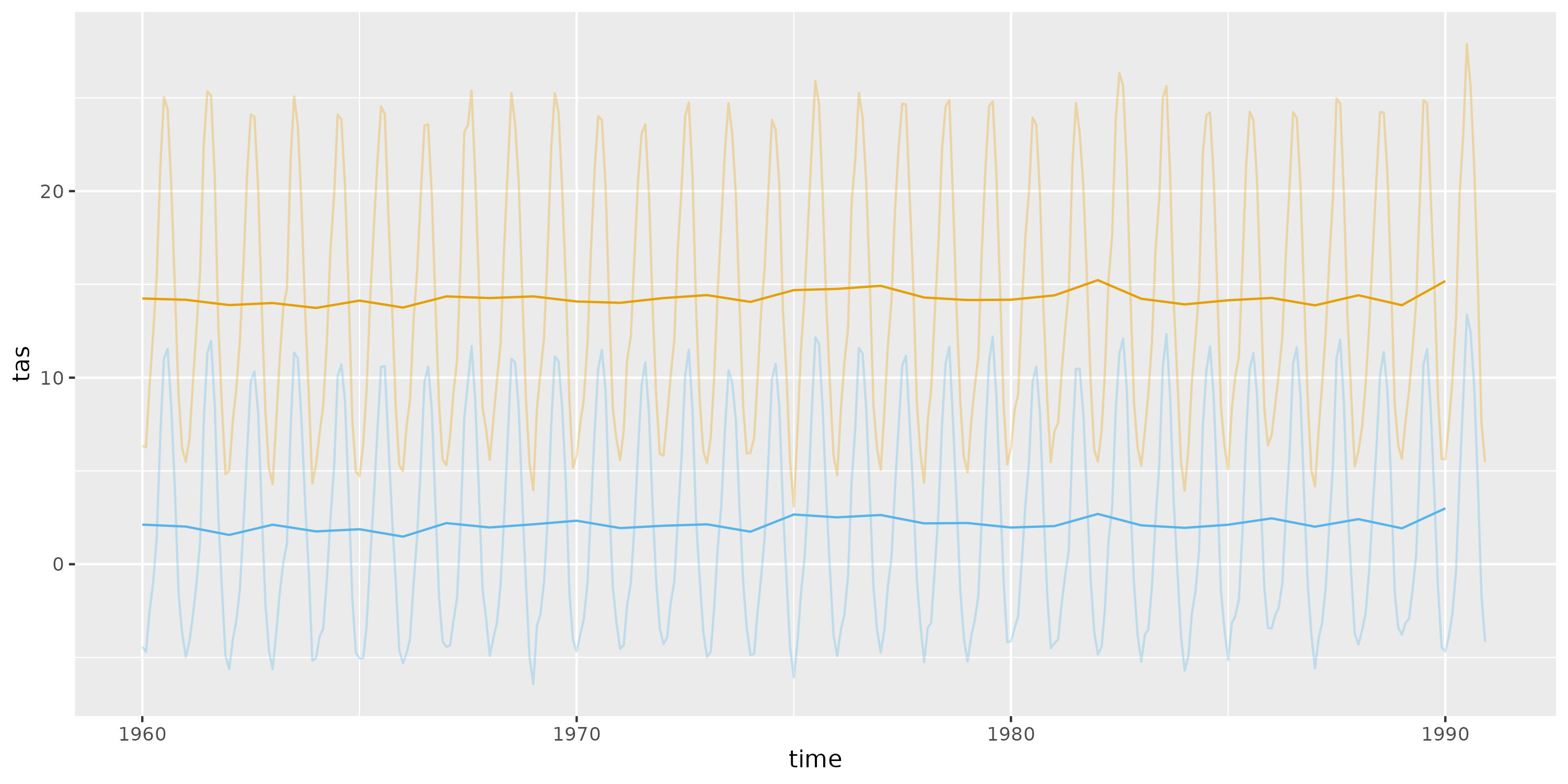
It is crucial to ensure a seamless transition between data from different sources when utilising climate data for past and future periods. This is important even when the overlapping period data source is the same. We have illustrated this concept through a graphical representation in this vignette. To exemplify, we will load the downscaled past climate data into R and extract a 30-year period (i.e., 1960-1990) in two locations.
library(dsclimtools)
library(stars)
library(units)
library(ggplot2)

point1 <- c(0, 41.5) %>% matrix(1, 2) %>% sf::st_point(dim = "XYZ")
point2 <- c(0, 42.8) %>% matrix(1, 2) %>% sf::st_point(dim = "XYZ")

past1 <- dsclimtools::read_dsclim("../data/dsclim",
                                  var = "tas",
                                  y_start = 10,
                                  y_end = 40,
                                  calendar_dates = TRUE,
                                  sf = point1,
                                  proxy = FALSE)

past2 <- dsclimtools::read_dsclim("../data/dsclim",
                                  var = "tas",
                                  y_start = 10,
                                  y_end = 40,
                                  calendar_dates = TRUE,
                                  sf = point2,
                                  proxy = FALSE)

figure <- ggplot() +
  geom_line(data = drop_units(as.data.frame(past1)),
                     aes(x = time,
                         y = tas),
                     color = "#E69F00",
                     alpha = 0.3) +
  geom_line(data = drop_units(as.data.frame(aggregate(past1,
                                                               by = calendar_dates(10, 41, "1 year"),
                                                               FUN = mean,
                                                               na.rm = TRUE))),
                     aes(x = time,
                         y = tas),
                     color = "#E69F00") +

  geom_line(data = drop_units(as.data.frame(past2)),
                     aes(x = time,
                         y = tas),
                     color = "#56B4E9",
                     alpha = 0.3) +
  geom_line(data = drop_units(as.data.frame(aggregate(past2,
                                                               by = calendar_dates(10, 41, "1 year"),
                                                               FUN = mean,
                                                               na.rm = TRUE))),
                     aes(x = time,
                         y = tas),
                     color = "#56B4E9")
Extracting future data in point locations for different climate change scenarios.
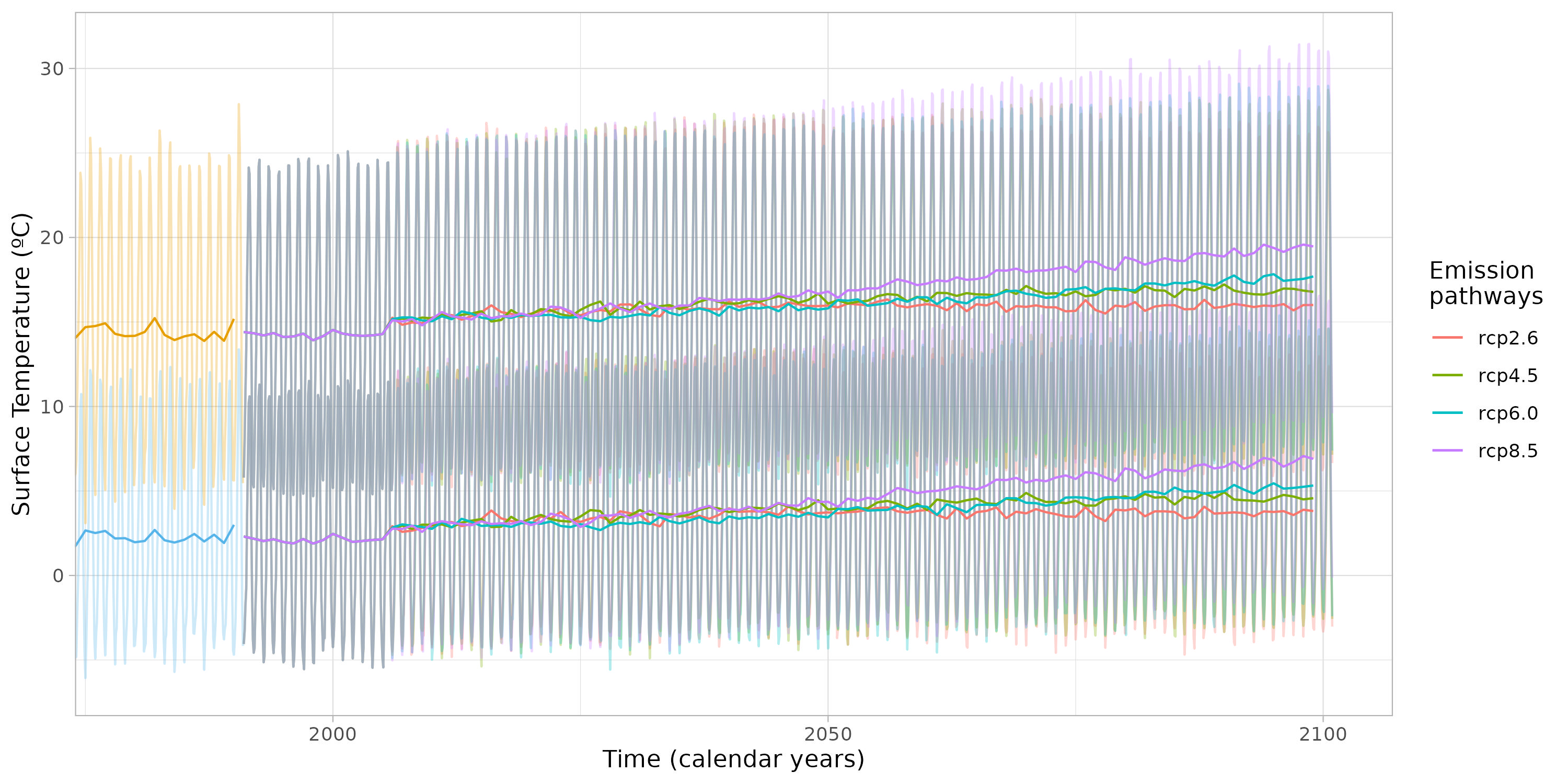
In this section, we present future climate data extracted from the same point locations for the various climate change scenarios. Furthermore, the data is aggregated on an annual basis in order to simplify any potential oscillations and provide a clearer visual representation.
rcps <- c("rcp2.6", "rcp4.5", "rcp6.0", "rcp8.5")
gcms <- c("CESM1-CAM5", "CSIRO-Mk3-6-0", "IPSL-CM5A-MR")

df <- expand.grid(gcms, rcps)

get_dscmip_point_data <- function(folder, var, start, end, rcp, gcm, sf, agg = NULL){
  data <- dsclimtools::read_dsclim(folder,
                                   var,
                                   start,
                                   end,
                                   rcp,
                                   gcm,
                                   calendar_dates = TRUE,
                                   sf,
                                   proxy = FALSE)

  if(!is.null(agg)){
    data <- aggregate(data,
                      by = calendar_dates(start,
                                          end,
                                          agg),
                      FUN = mean,
                      na.rm = TRUE)
  }

  data <- as.data.frame(data)
  data$gcm <- gcm
  data$rcp <- rcp
  data
}

fut1 <- mapply(get_dscmip_point_data,
               rcp = df$Var2,
               gcm = df$Var1,
               MoreArgs = list(folder = "../data/dsclim",
                               var = "tas",
                               start = 41,
                               end = 150,
                               sf = point1),
               SIMPLIFY = FALSE)
fut1 <- do.call(rbind, fut1)

fut1.agg <- mapply(get_dscmip_point_data,
                   rcp = df$Var2,
                   gcm = df$Var1,
                   MoreArgs = list(folder = "../data/dsclim",
                                   var = "tas",
                                   start = 41,
                                   end = 150,
                                   sf = point1,
                                   agg = "1 year"),
                   SIMPLIFY = FALSE)
fut1.agg <- do.call(rbind, fut1.agg)

fut2 <- mapply(get_dscmip_point_data,
               rcp = df$Var2,
               gcm = df$Var1,
               MoreArgs = list(folder = "../data/dsclim",
                               var = "tas",
                               start = 41,
                               end = 150,
                               sf = point2),
               SIMPLIFY = FALSE)
fut2 <- do.call(rbind, fut2)

fut2.agg <- mapply(get_dscmip_point_data,
                   rcp = df$Var2,
                   gcm = df$Var1,
                   MoreArgs = list(folder = "../data/dsclim",
                                   var = "tas",
                                   start = 41,
                                   end = 150,
                                   sf = point2,
                                   agg = "1 year"),
                   SIMPLIFY = FALSE)
fut2.agg <- do.call(rbind, fut2.agg)

figure <- figure +
  stat_summary(data = drop_units(fut1),
               aes(x = time,
                   y = tas,
                   group = rcp,
                   color = rcp),
               fun = mean,
               geom = 'line',
               alpha = 0.3) +
  stat_summary(data = drop_units(fut1.agg),
               aes(x = time,
                   y = tas,
                   group = rcp,
                   color = rcp),
               fun = mean,
               geom = 'line') +

  stat_summary(data = drop_units(fut2),
               aes(x = time,
                   y = tas,
                   group = rcp,
                   color = rcp),
               fun = mean,
               geom = 'line',
               alpha = 0.3) +
  stat_summary(data = drop_units(fut2.agg),
               aes(x = time,
                   y = tas,
                   group = rcp,
                   color = rcp),
               fun = mean,
               geom = 'line') +
  theme_light() +
  labs(y = "Surface Temperature (ºC)",
       x = "Time (calendar years)") +
  coord_cartesian(xlim = as.Date(c('1980-01-01','2100-12-31'))) +

  scale_color_discrete(name = "Emission\npathways",
                       guide = "legend")

figure
The objective of this plot is to demonstrate the gradual transition between past and future data, as well as the divergence between the various climate change scenarios.