3. Downscaling with crossvalidation
Source:vignettes/a3_Downscale_with_Cross-validation.Rmd
a3_Downscale_with_Cross-validation.RmdHere, we document the downscaling process with crossvalidation of Trace-21ka paleoclimate data using the UERRA dataset for the historical period. This evaluation allows us to test several configurations of the downscaling process and select the optimal ones to run the downscaling of the whole dataset.
More information can be found here, here, and here.
Downscaling
The downscaling process will be divided in several steps.
Defining variables and folds for crossvalidation
Let start by loading the R package dsclim. Then, we
create a vector (vars) containing the names of several
climate variables to be used as predictors in the downscaling process.
The variable local.var is assigned the value “tasmin”,
which is the variable that we aim to downscale in the first place. The
next line creates a list of six elements containing the years 1961 to
1990 split into five-year groups, this is where we are defining the
years to be used in the crossvalidation. To do so, we will fit one
downscaling model for each of the five years period using data from the
rest of the years and using this period to evaluate/validate the model.
Hence, we will fit six models. Finally, the trace.dir
variable is set to the path of a directory containing TraCE21ka
data.
Defining parameters for downscaling
The following code is setting up parameters for the R package
downscaleR. The spatial.pars list is defining
the variables that should be combined using a Principal Component
Analysis. Here, we specify all predictor variables. Hence, those models
using spatial.pars argument will use all the variables to fit a PCA and
transform the varibles. More especifically, the PCA will retain those
axis that explain up to 90% of the variance (v.exp) and
will not be rotated. The local.pars.XXX objects define
different configurations of local vars for the models. M2
models use the only one variable as the local variable, whereas
M3 uses all predictor variables as local variables.
Finally, models ending in 1 use the information of the local pixel as
predictor, whereas models ending in 4 use the information from the 4
closest pixels as predictors.
Data loading
To load the data, we retrieve file names from all files in the trace directory. The first line assigns the trace file names from the trace directory to the variable “trace.file.names”. Then, we loads the trace files into the variable “hist.trace” and specifies the years 1961-1990, since we are not intended to downscale the whole period but only the historical period to run the crossvalidation. The following lines check that the data were loaded properly.
trace.file.names <- traceFileNames(trace.dir)
hist.trace <- dsclim::loadTrace(trace.file.names, years = 1961:1990)
hist.trace$Variable$varName
head(hist.trace$Dates[[1]]$start)
tail(hist.trace$Dates[[1]]$start)
head(hist.trace$Dates[[1]]$end)
tail(hist.trace$Dates[[1]]$end)
Now, we need to load the data from the UERRA project since this is
going to be our current high resolution climate data to be used as
predictand. The first line is loading the local variable
(local.var) from the
2m_temperature/latlon/1961-90_2m_tmin.nc file in the
UERRA-HARMONIE directory and and assigning it to the variable
uerra.data. The following lines just check that data were
loaded properly and matches the same dates than loaded TraCE21ka
data.
Downscaling
Now, we can start fitting models with the cross validation approach.
In general, the code uses the downscaleR package to fit
a Generalized Linear Model (GLM) downscaling method to create a model
that predicts paleoclimate data from historical climate. The
family argument sets the distribution of the model to a
Gaussian distribution with an identity link. The
folds argument sets the number of folds to use in the
cross-validation. The prepareData.args is a list of
arguments that sets the global, local, and spatial predictors to use in
the model.
The result from the downscaling is a high resolution dataset for the
whole period (1961-1990), although the data for group of five years were
not used to fit the particular model used to dowscale this five years
data. Finally, we use the spatialPlot function from the
visualizeR package to plot an average of the output (e.g. a
climatology calculated with the transformeR
package).
To see the code for each model, select a tab:
This model uses spatial pars but do not use global or local variables.
GLM.1.sp <- downscaleR::downscaleCV(
  x = hist.trace,
  y = uerra.data,
  method = "GLM",
  family = gaussian(link = "identity"),
  folds = folds,
  prepareData.args = list(
    global.vars = NULL,
    local.predictors = NULL,
    spatial.predictors = spatial.pars,
    combined.only = TRUE
  )
)

visualizeR::spatialPlot(transformeR::climatology(GLM.1.sp))
This model uses a local variables with 1 local pixel, but no spatial or global variables.
GLM.21 <- downscaleR::downscaleCV(
  x = hist.trace,
  y = uerra.data,
  method = "GLM",
  family = gaussian(link = "identity"),
  folds = folds,
  prepareData.args = list(
    global.vars = NULL,
    local.predictors = local.pars.M21,
    spatial.predictors = NULL
  )
)

visualizeR::spatialPlot(transformeR::climatology(GLM.21))
This model uses a local variables with 1 local pixel and spatial variables, but no global variables.
GLM.21.sp <- downscaleR::downscaleCV(
  x = hist.trace,
  y = uerra.data,
  method = "GLM",
  family = gaussian(link = "identity"),
  folds = folds,
  prepareData.args = list(
    global.vars = NULL,
    local.predictors = local.pars.M21,
    spatial.predictors = spatial.pars,
    combined.only = TRUE
  )
)

visualizeR::spatialPlot(transformeR::climatology(GLM.21.sp))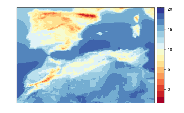
This model uses a local variables with 4 local pixel, but no spatial or global variables.
GLM.24 <- downscaleR::downscaleCV(
  x = hist.trace,
  y = uerra.data,
  method = "GLM",
  family = gaussian(link = "identity"),
  folds = folds,
  prepareData.args = list(
    global.vars = NULL,
    local.predictors = local.pars.M24,
    spatial.predictors = NULL
  )
)

visualizeR::spatialPlot(transformeR::climatology(GLM.24))
This model uses a local variables with 4 local pixel and spatial variables, but no global variables.
GLM.24.sp <- downscaleR::downscaleCV(
  x = hist.trace,
  y = uerra.data,
  method = "GLM",
  family = gaussian(link = "identity"),
  folds = folds,
  prepareData.args = list(
    global.vars = NULL,
    local.predictors = local.pars.M24,
    spatial.predictors = spatial.pars
  )
)

visualizeR::spatialPlot(transformeR::climatology(GLM.24.sp))
This model uses all variables as local variables with 1 local pixel, but no spatial or global variables.
GLM.31 <- downscaleR::downscaleCV(
  x = hist.trace,
  y = uerra.data,
  method = "GLM",
  family = gaussian(link = "identity"),
  folds = folds,
  prepareData.args = list(
    global.vars = NULL,
    local.predictors = local.pars.M31,
    spatial.predictors = NULL
  )
)

visualizeR::spatialPlot(transformeR::climatology(GLM.31))
This model uses all variables as local variables with 4 local pixel, but no spatial or global variables.
GLM.34 <- downscaleR::downscaleCV(
  x = hist.trace,
  y = uerra.data,
  method = "GLM",
  family = gaussian(link = "identity"),
  folds = folds,
  prepareData.args = list(
    global.vars = NULL,
    local.predictors = local.pars.M34,
    spatial.predictors = NULL
  )
)

visualizeR::spatialPlot(transformeR::climatology(GLM.34))
Evaluate downscaling performance
Now that we have a downscaled version of the data, we can evaluate their values against the “real” data, represented here by the UERRA dataset.
Create function to extract info
First, we define a function that will run the evaluation and extract significant metrics.
Run evaluation
Then, we can use this function to evaluate all the models. To speed
things up, we run this code in several cores of the computer using the
parallel package.
ds.methods <- c("GLM.1.sp", "GLM.21", "GLM.21.sp", "GLM.24", "GLM.24.sp", "GLM.31", "GLM.34")

value.indices <- c("Mean", "sd", "Skewness")

library(parallel)

cl <- makeCluster(detectCores())

clusterExport(cl, c("ds_validation", ds.methods, "uerra.data", "value.indices"))

val.results <- parLapply(
  cl,
  value.indices,
  function(i, j, k, l) {
    ds_validation(
      models = j,
      obs = k,
      measure.code = l,
      index.code = i
    )
  },
  ds.methods,
  uerra.data,
  "bias"
)

stopCluster(cl)

names(val.results) <- value.indices
Plot evaluations’ results
Finally, we can plot the results from the evaluations in several formats.
Error (or bias) maps
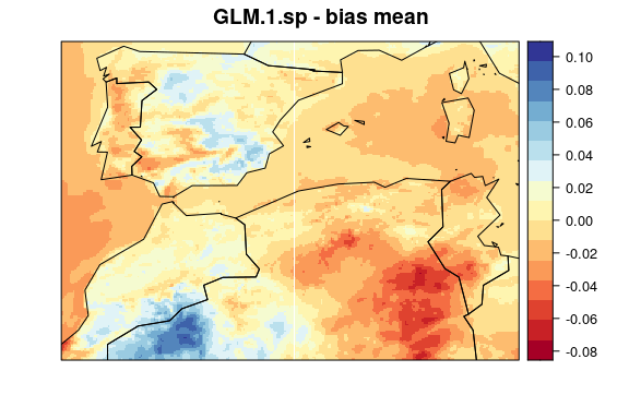
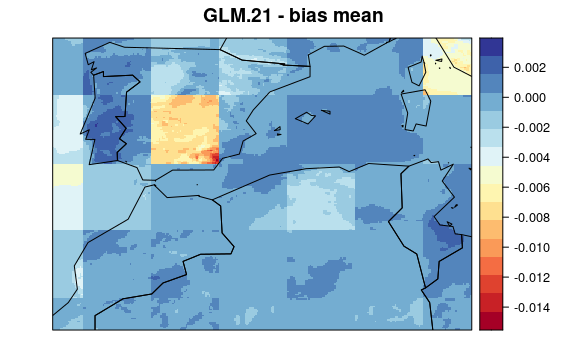
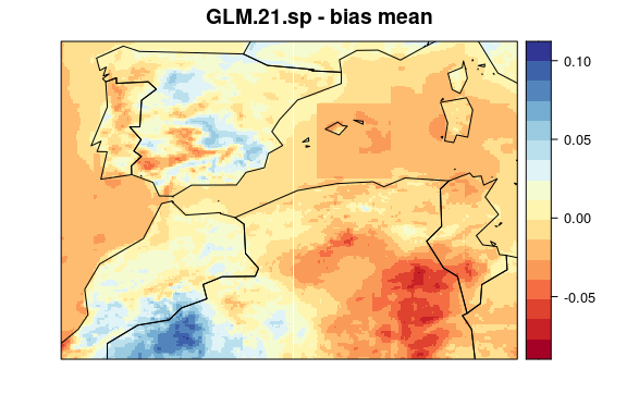
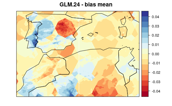
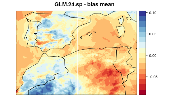
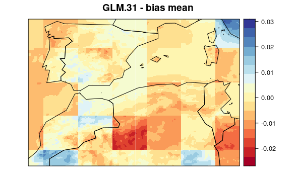
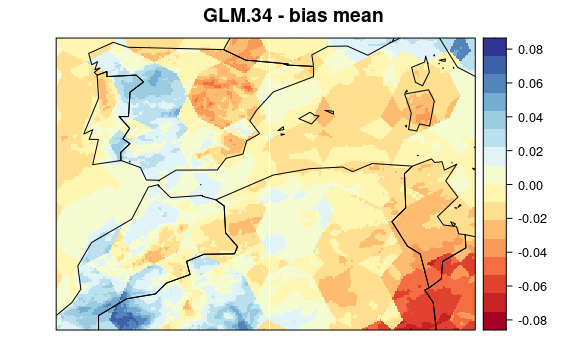
First, we plot mean bias in each pixel (the mean include 30 years * 12 months data). To see the maps from each model select a tab:
visualizeR::spatialPlot(val.results[[1]][[1]],
  backdrop.theme = "countries",
  main = "GLM.1.sp - bias mean"
)
visualizeR::spatialPlot(val.results[[1]][[2]],
  backdrop.theme = "countries",
  main = "GLM.21 - bias mean"
)
visualizeR::spatialPlot(val.results[[1]][[3]],
  backdrop.theme = "countries",
  main = "GLM.21.sp - bias mean"
)
visualizeR::spatialPlot(val.results[[1]][[4]],
  backdrop.theme = "countries",
  main = "GLM.24 - bias mean"
)
visualizeR::spatialPlot(val.results[[1]][[5]],
  backdrop.theme = "countries",
  main = "GLM.24.sp - bias mean"
)
visualizeR::spatialPlot(val.results[[1]][[6]],
  backdrop.theme = "countries",
  main = "GLM.31 - bias mean"
)
visualizeR::spatialPlot(val.results[[1]][[7]],
  backdrop.theme = "countries",
  main = "GLM.34 - bias mean"
)
Violin plots sumarizing results
To have an overall perspective of all the metrics from the different models, we can use violin plots for each model and the three metrics of the bias (mean, sd, and skewness).
library(reshape2)
library(ggplot2)
getGridData <- function(grid) grid$Data

test <- lapply(val.results, FUN = function(x) lapply(x, getGridData))

test <- melt(test)

test$mean <- ave(test$value, as.factor(test$L1), as.factor(test$L2), FUN = mean)

test$L2 <- factor(test$L2, levels = ds.methods)
test$L1 <- factor(test$L1, levels = value.indices)

ggplot(test, aes(x = L2, y = value)) +
  geom_violin(aes(fill = mean)) +
  facet_grid(L1 ~ ., scales = "free")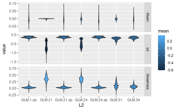
Error or bias histograms
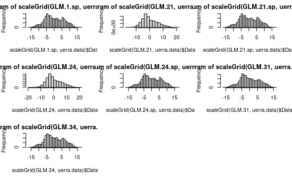
Finally, we complement previous evaluations ploting the histograms from each metric.
library(transformeR)
par(mfrow = c(3, 3))
hist(scaleGrid(GLM.1.sp, uerra.data)$Data)
hist(scaleGrid(GLM.21, uerra.data)$Data)
hist(scaleGrid(GLM.21.sp, uerra.data)$Data)
hist(scaleGrid(GLM.24, uerra.data)$Data)
hist(scaleGrid(GLM.24.sp, uerra.data)$Data)
hist(scaleGrid(GLM.31, uerra.data)$Data)
hist(scaleGrid(GLM.34, uerra.data)$Data)